2026-11-12 · 25 min · 3d · looped-transformers · vision-transformers · point-cloud · benchmarks
A 4:49 narrated explainer, drawn in code. Every number and picture in it is this article's own; the sources are below.
› transcript
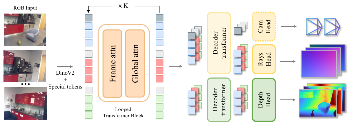
VGGT stacks twenty-four pairs of different blocks to rebuild a scene from photos. What if one pair, run again and again, did the same job? Hi, I'm Oswin! Déjà View rebuilds a scene by running the same block over and over. Let's open it up. Chapter one. Photos in, geometry out. Hand the model photos from different angles. An encoder turns each one into patch tokens. VGGT pushes them through twenty-four pairs of different blocks. Frame attention looks within one photo; global attention looks across all of them. Heads read out depth maps, point maps and cameras. Accuracy grew with size: VGGT has one point two six billion parameters. Here is the job, from NVIDIA's post. Drone footage goes in; a point cloud and the camera's path come out. Chapter two. One block, sixteen times. Deep stacks seem to refine their answer layer by layer. So make that explicit: one shared block, applied K times to the same tokens. The paper's diagram. Encoder tokens on the left, two shallow decoders on the right. In the middle, one block, frame then global attention, fed back into itself K times. Each loop reads the whole state, every token of every view, and writes a refined one. Decode it after two loops: the room is smeared, the cameras far off. After four, the walls start to line up. After eight, the cameras are close. After sixteen, sharp geometry and accurate cameras. Training only ever checks the last step. Inside, an ordinary block with three dials. Attention, then an MLP, each added with a scale per channel. The scales come from a tiny network that reads where this step starts and ends in time. That is how one block tells an early step from a late one. Then a state gate scales everything. In the released weights it sits below one, so older content fades. I counted the checkpoint's tensors. Three quarters is the encoder, eighty-six point six million, run once per photo. The block doing the multi-view reasoning is fourteen and a half million, run sixteen times. Two shallow decoders read out depth and rays. One hundred and seventeen million in all. Untied, sixteen copies would make it about three hundred and twenty-nine million. Chapter three. Turning the dial. One checkpoint serves every loop count from eight to sixteen. Each batch draws a loop count between eight and sixteen, favouring the high end. The gates read time, not a step number, so one set of weights fits every count. Only the final state is scored. Want fewer loops? You could stop the sixteen-step schedule early. Or run K steps on a K-step time grid. That wins at every budget. At eight loops, pose AUC at three degrees is zero point four three, against zero point three one for stopping early. Now the bill. Ten times fewer parameters is not ten times fewer FLOPs: half or less of Pi3 and VGGT, about the same as Depth Anything 3 Large. Why so close? Count one loop. The linear layers cost under one teraflop. Frame attention is cheap: each photo sees only its own tokens. Global attention is three of the four teraflops, every token looking at all thirty-one thousand. Sharing weights does not touch that. Chapter four. Does it hold up? A sign the loop does real work: one patch's global attention onto another view, loop by loop. It starts diffuse and settles on the matching point, though training never asked for matches. And the limit. Past sixteen loops the state drifts; past about thirty steps, it collapses. What I found checking the claims. It leads the averages, an inlier ratio of eighty point three, but wins few single cells against the concurrent VGGT Omega. Shared beat untied blocks, but only in half-length runs. And the quick-start script runs twelve loops; the tables use sixteen. Tying weights shrinks parameters, not FLOPs. And the loop count is a real dial, above all for precise camera poses. To recap. One shared block, looped. Most parameters are the encoder. For fewer loops, re-grid; don't stop early. Every source is in the full article. I'm Oswin. Bye!
Why read this
Notabletop 60%Déjà View's looped block from paper, code and checkpoint: where the 117M parameters sit, the gates per step, and a FLOP model that lands near Table 3.
- Original analysis
- Runs on a consumer GPU
- A lasting reference
3D & spatialMixed licencesResearch paper
How this was scored
- Is it new?
- 2 of 3: A real new idea, method or capability
- Can I trust it?
- 2 of 3: Measures key facts from files, code or configs
- Can I run it?
- 2 of 3: Open code or weights with real limits
- Will I understand it?
- 2 of 3: Mechanism from first principles with figures
- Can I act on it?
- 2 of 3: A concrete recipe, numbers or comparison
- Will it last?
- 2 of 3: A reference for a year or more
- Does it affect many?
- 1 of 3: A specialist community
- Only here?
- 2 of 3: A teardown or measurement few others did
Score 67 of 100, ranked 232 of 740 rated articles. Each question is answered 0–3 by hand, and a 3 is rare. How articles are scored
Every feed-forward reconstruction model of the last two years has grown the same way. DUSt3R had a ViT-Large encoder and a ViT-Base decoder. VGGT has 1.26 billion parameters. Depth Anything 3's giant variant has 1.2 billion. The accuracy went up with the size, so nobody asked whether the size was doing what we thought.
Déjà View, from NVIDIA's Dynamic Vision and Learning group with Modena, Toronto and ETH Zürich (a NeurIPS 2026 oral), asks it. Its answer is a model with one transformer block (a frame-attention and global-attention pair) where VGGT stacks 24 such pairs, applied over and over to the same tokens. The whole thing is 117 million parameters and it leads the five-benchmark averages against models eight to ten times its size.
I read the paper, the code and the header of the released checkpoint. The parameter story is real and more lopsided than the headline. The compute story is narrower than "comparable or less" suggests, and it is narrower for a reason that is easy to see once the FLOPs are written out: weight tying saves parameters, and loops cost FLOPs.
What a feed-forward reconstructor has to produce
Start from the classical pipeline, because the new models are trying to delete it. Structure-from-motion matches keypoints across photos, estimates relative poses, triangulates points, and runs bundle adjustment: a nonlinear least-squares solve that nudges every camera and point until reprojection error stops falling. It is iterative by construction, and it falls apart on blank walls, repeated facades and moving things.
DUSt3R replaced that with a network that takes two images and regresses a pointmap for each: an array giving, for every pixel, its 3D position in the first camera's frame. Camera pose and intrinsics fall out of the pointmap by fitting. Two views at a time means a scene of photos needs many pairs and a global alignment step afterwards, which is where MASt3R-SfM spends its time.
VGGT took all views at once. Each image becomes DINOv2 patch tokens, plus a camera token and a few register tokens. The tokens then pass through a stack that alternates two kinds of attention:
- frame attention, where each view's tokens attend only to themselves;
- global attention, where every token of every view attends to every other token in the set.
Heads on top decode depth maps, pointmaps and camera parameters. VGGT runs 24 frame blocks and 24 global blocks at width 1024. Pi3, MapAnything and Depth Anything 3 are variations on this skeleton. I've covered several of the descendants on this site: HiP3R stitching long videos from local reconstructions, R³ and AMB3R-SLAM streaming on a frozen Depth Anything 3, SplatAnything putting a Gaussian head on one, and in today's 3D reconstruction roundup, Click3R letting a user correct DUSt3R with clicks.
Déjà View outputs a slightly different thing from a pointmap. For each image it predicts a depth map and a six-channel ray map : an origin and a direction per pixel. A world point is then
and camera rotation, translation and intrinsics are fitted from the rays,
following Depth Anything 3. The code computes exactly this in _decode:
pred_points = pred_rays[..., 3:6] + pred_rays[..., :3] * pred_depth.
The evaluation aligns the predicted points to ground truth with a similarity transform (Sim(3): rotation, translation, scale) and reports:
- Rel. L2, the mean of over valid points;
- inlier ratio (IR), the share of points whose relative error is under 3%;
- pose AUC@3° and AUC@30°, the area under the cumulative curve of per-pair angular pose error up to 3° and up to 30°.
AUC@30 is forgiving. AUC@3 is where a model has to get cameras nearly exactly right, and it is where the models separate.
Depth that might be iteration in disguise
The paper's hypothesis comes from two earlier probes. Starý and colleagues decoded DUSt3R's intermediate layers and found the pointmap getting better layer by layer, as if each layer were one more step of a refinement, even though every layer has its own weights. RAPTOR (Jacobs et al., ICLR 2026) showed the layers of a trained ViT can be approximated by a few blocks looped.
If a stack of different layers is mostly doing the same refinement repeatedly, the different weights are paying for iteration with unique parameters. Déjà View makes the iteration the architecture: one block, applied times, to a state that starts as DINOv2 features.
Language models have been looping for a while: see what separates Ouro from Huginn and SMELT's compute-matched comparison. Déjà View is the first I've read that does it for multi-view geometry at full benchmark scale.
The block
The looped block is two sub-blocks in sequence, VGGT-style: frame attention with 2D rotary position embeddings, then global attention over all views' tokens. Each sub-block is the standard pre-norm attention plus MLP, with LayerScale, and with three extra channel-wise scales the paper calls gates:
The gates come from a small MLP fed with sinusoidal embeddings of two numbers, and : where this step starts and where it lands on a time axis. The MLP's last layer is zero-initialised, so at the start of training every gate is exactly 1 and the block is a plain transformer block. The design is RAPTOR's; the difference is that Déjà View trains the block end to end on the reconstruction loss, with no teacher.
Conditioning on an interval of continuous time, instead of a step index, is what lets one set of weights serve different step counts. Step 6 of 12 and step 8 of 16 are both "from 0.45 to 0.55 of the way", roughly, and the block sees them as the same kind of step.
The code is short enough to quote. This is the whole inference loop, from
src/dvlt/model/dvlt/model.py:
def _solve_inference_linspace_k(self, x, rope_pos, B, S):
    """Inference for k_sampling='linspace': uniform grid with configurable K."""
    K = self.inference_steps
    ts = torch.linspace(0.0, 1.0, K).tolist()
    for i in range(K):
        t_now = ts[i]
        t_next = ts[i + 1] if i + 1 < K else 1.0
        x = self._interval_step(x, t_now, t_next, rope_pos, B, S)
    return x
One detail differs from the paper. Section 3.4 writes the grid as
, so steps cover equal intervals ending at 1. The code uses
linspace(0, 1, K), which gives points, so step starts at
and the last step is conditioned on the degenerate interval
. The docstring calls it a "terminal-step sentinel". It is trained that
way too, so it is consistent, but if you reimplement from the paper you will
build a slightly different model.
Supervision lands only on the final state. RAFT-style refiners decode and penalise every step; Déjà View decodes once, which saves decoder passes per training step. Whether the intermediate states are any good is then an empirical question, and the answer, further down, is "decodable but not optimal".
Where the 117 million parameters sit
The checkpoint is one model.safetensors file. Its header lists every tensor
and its shape, so I fetched the 40,920-byte header with an HTTP range request
and summed the shapes. The total is 117,081,731, which matches both the paper's
117M and the Hugging Face API's count.
| Part | Parameters | Share |
|---|---|---|
| DINOv2 ViT-B/14 encoder (12 layers, width 768) | 86,582,016 | 74% |
| The looped block (frame + global sub-block) | 14,495,424 | 12.4% |
| … of which the six gates' MLPs | 316,096 | 0.3% |
| Depth decoder (2 blocks at width 384, conv head) | 11,401,506 | 9.7% |
| Ray decoder (2 blocks at width 384) | 4,298,264 | 3.7% |
| Camera head, camera and register tokens | 304,521 | 0.3% |
Three-quarters of the model is the encoder, which runs once per image. The part that does the multi-view reasoning, the part the paper is about, is 14.5 million parameters. That is less than two of VGGT's 48 aggregator blocks, which at width 1024 with a 4x MLP are about 12.6 million each.
The paper's ablation compares this against a "decoupled" model with 16 independent blocks and no gates. On the same layer shapes, 16 ungated copies are 226.9 million parameters, so the decoupled model is about 329 million in total. Same FLOPs, almost three times the parameters.
What the gates do, step by step
The gate MLPs are small, 1.3 MB of float32 for both sub-blocks together, so I range-fetched just those tensors and the LayerScale vectors from the checkpoint and evaluated the gate network myself in NumPy for every step of , 12 and 16, using the code's own time grid. The widget plots the channel means.
The paper reports neither of the following.
First, is below 1 on average at every step. Each application multiplies the state by about 0.73 to 0.93 per channel (channel mean) in the frame sub-block and about 0.86 in the global sub-block, then adds the attention and MLP updates on top. The recurrence is a leaky accumulator: older contributions decay and new ones are added. The paper's Figure 3 shows the state norm growing anyway, so the updates outrun the decay.
Second, the two sub-blocks use time very differently. The frame sub-block's climbs steadily from 0.73 at to 0.93 at the end: early steps forget more of the state, late steps keep it. The global sub-block's barely moves (0.863 to 0.869), and only its attention gate drifts, from 0.77 down to 0.67. The time-dependence lives mostly in the per-view part of the loop.
That bears on Solv3R, which fine-tunes this exact checkpoint and argues that a step-conditioned block cannot be continued past its schedule. The gates are where that conditioning lives. A state gate that moves from 0.73 to 0.93 between the first step and the last is not cosmetic; it changes what an "extra" step does to the state.
These are means over 768 channels. In the frame sub-block, individual channels of the state gate range from 0.02 to 1.33, so a handful of channels are being nearly reset each step and a handful amplified. I don't have activations, only weights, so I can't say which channels carry what.
One checkpoint, any K from 8 to 16
Training samples the step count per batch. The code draws , scales it to and rounds. Beta(2, 1) has density , so large is favoured; the expected value is steps. The draw is seeded identically on every rank so all 128 GPUs run the same in a batch and nobody waits.
There are two ways to spend less than 16 steps at inference, and the paper's Appendix E compares them:
- Early exit: run the 16-step schedule and decode the state after step .
- Re-gridded K: run steps on a -point time grid, so every step knows it is one of .
Re-gridding wins at every budget, and the gap is largest at the smallest one. Figure 8 averages the five benchmarks. I read its values from the SVG's own path coordinates rather than by eye. Its 16-step AUC@3, 0.567, sits a little under the 57.2 I get by averaging Table 2 (the appendix's Table 8 says 56.8), so the figure probably averages slightly differently; the gaps are under a point.
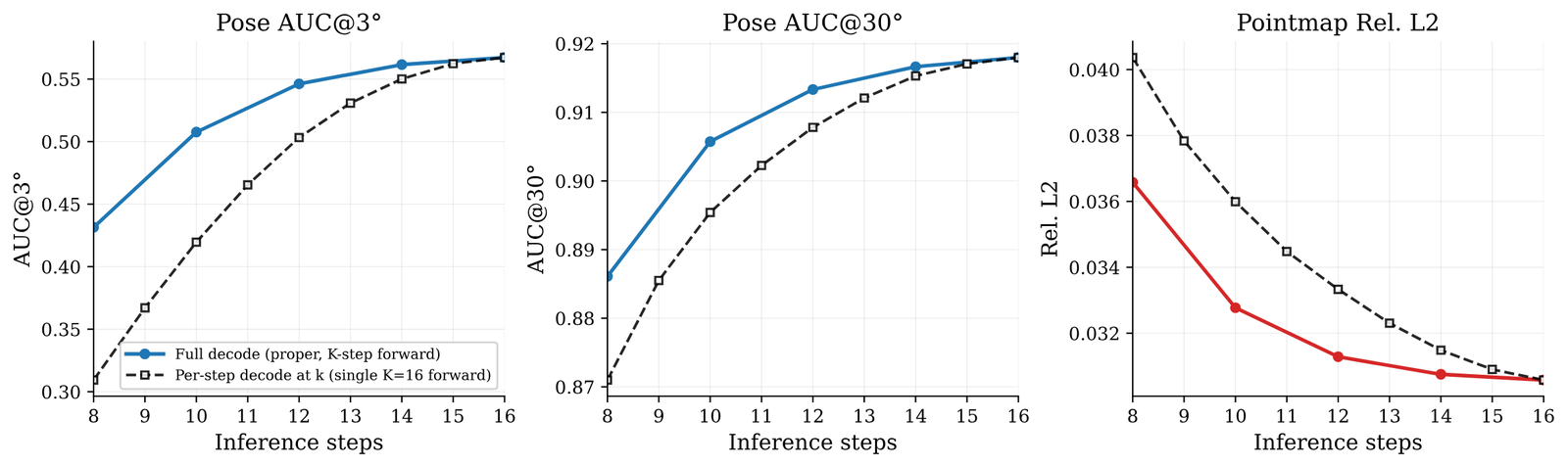
| Steps | AUC@3, re-gridded | AUC@3, early exit | AUC@30, re-gridded | Rel. L2, re-gridded |
|---|---|---|---|---|
| 8 | 0.431 | 0.309 | 0.886 | 0.0366 |
| 10 | 0.508 | 0.420 | 0.906 | 0.0328 |
| 12 | 0.546 | 0.503 | 0.913 | 0.0313 |
| 14 | 0.562 | 0.550 | 0.917 | 0.0308 |
| 16 | 0.567 | 0.567 | 0.918 | 0.0306 |
The text of Appendix E says AUC@3 at rises "from 0.31 to 0.44"; the figure's own coordinates put the re-gridded point at 0.431. Small, but the text rounds in its own favour.
AUC@30 is close to saturated by . AUC@3, the precise-pose metric, is not: it gains 14 points of AUC between 8 and 16 steps. If you need cameras accurate to a degree or two, the extra loops are worth paying for. If you need a roughly right point cloud, half of them are.
The released code has a trap here. The DVLT wrapper class defaults to
inference_steps=12, and the checkpoint's config.json says 12 as well. The
README's quickstart builds DVLT(img_size=504) and so runs 12 loops, not the
16 behind every table. The Hydra path used by python -m dvlt.scripts.test
passes inference_steps: None from DVLTModelConfig, which falls through to
16. That is my reading of the code; I didn't run it. It fits the README's
reference table for the scripts.test path, whose pose AUCs (AUC@3 of 0.8319 on DTU
and 0.4340 on nuScenes) round to Table 2's 16-step numbers. Same
weights, two defaults. Pass inference_steps=16 if you want the paper's
numbers.
The compute bill
Here is the claim to check: Déjà View matches or beats much larger models "at comparable or lower compute". The paper's Table 3 measures forward-pass FLOPs on an A100 with 24 input views:
| Model | Params (M) | TFLOPs, 24 views | vs Déjà View | Avg IR | Avg AUC@30 |
|---|---|---|---|---|---|
| Déjà View | 117 | 75.9 | 1.00x | 80.3 | 91.8 |
| DA3-L | 356 | 71.4 | 0.94x | 58.3 | 79.7 |
| VGGT-Ω-1B | 1,144 | 99.8 | 1.31x | 74.8 | 90.7 |
| MapAnything | 1,228 | 148.4 | 1.96x | 69.0 | 83.3 |
| Pi3 | 959 | 153.8 | 2.03x | 77.4 | 88.6 |
| DA3-G | 1,201 | 178.7 | 2.35x | 66.5 | 84.7 |
| VGGT | 1,257 | 190.0 | 2.50x | 66.0 | 84.0 |
The ratio column is my division. Pi3 needs 153.8 TFLOPs for the same 24 views and VGGT needs 190.0, so against the billion-parameter models Déjà View uses half or less of the compute, which is a real saving. Against DA3-L it uses 6% more and is far more accurate. Against the concurrent VGGT-Ω it saves a quarter. "Comparable or lower" is accurate; "ten times smaller" is about parameters only. The project page claims "1.9–2.3× less compute" and names Pi3 and DA3-G, which by Table 3 come to 2.03x and 2.35x. The range is conservative rather than wrong.
Why is the saving in parameters so much larger than the saving in FLOPs? Write the cost out. I assumed square 504-pixel inputs (36 × 36 patches, plus 1 camera and 4 register tokens, so 1,301 tokens per view) and counted two FLOPs per multiply-add:
- the linear layers of one looped step cost 0.88 TFLOPs at 24 views;
- frame attention's score-and-mix costs 0.12 TFLOPs, because each view only sees its own 1,301 tokens;
- global attention's costs 3.00 TFLOPs, because each of 31,224 tokens sees all 31,224.
That is 4.0 TFLOPs per loop, three-quarters of it global attention. Sixteen loops are 64.0, the DINOv2 encoder is another 6.8 and the two decoders' transformer blocks 0.7, which sums to 71.6. The paper measures 75.9; the remaining 4.3 is plausibly the convolutional depth head, which upsamples to full resolution and which I did not model. The same counting gives VGGT's backbone 175.6 TFLOPs against its measured 190.0, so the method lands near the paper's numbers twice. It is a model, not a measurement; the resolution in particular is my assumption.
What it shows is the shape of the bill. Compute is set by how many global attention layers run and how wide they are. Déjà View runs 16 at width 768; VGGT runs 24 at width 1024. By my count that is a little under half of VGGT's global attention work, and it is most of the 2.5x. Parameters don't enter into it. Tying the weights made the model small; it did nothing for the FLOPs, and the paper is careful to say "comparable" rather than "lower" for that reason.
Table 3 is also a single point: 24 views. The global term grows with the square of the view count, so at 100 views it dominates even more, and every model in the table pays the same quadratic. Peak memory is the other number in Table 3 that favours Déjà View: 4.9 GiB at 24 views against 14.7 for VGGT. Every model holds about one layer's activations at a time at inference, so the gap is more likely weights and width: VGGT's 1,257M parameters are about 4.7 GiB in fp32 against under 0.5 GiB here, and its tokens are 1024 wide, not 768.
The dial uses only printed points for accuracy: Figure 8's five re-gridded budgets, with the early-exit value beside each, and the baselines' averages from Tables 1 and 2. The FLOPs for below 16 are my model: 75.9 minus 4.0 per loop removed. At that is about 43.9 TFLOPs, and the re-gridded model's AUC@30 of 0.886 matches Pi3's average of 88.6 at under a third of Pi3's compute. Its AUC@3, 0.431, sits below Pi3's 45.2 and above VGGT's 39.5. Its Rel. L2, 0.0366, is worse than Pi3's 0.0334. One knob, three different answers depending on which metric you care about.
Five benchmarks, cell by cell
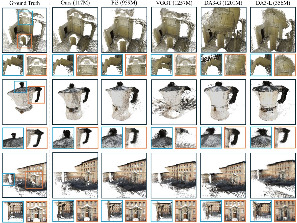
The benchmarks span object-centric scans (DTU), outdoor scenes (ETH3D), small indoor rooms (7-Scenes), larger indoor scans (ScanNet++, with a scene-level split from its training data) and driving (nuScenes).
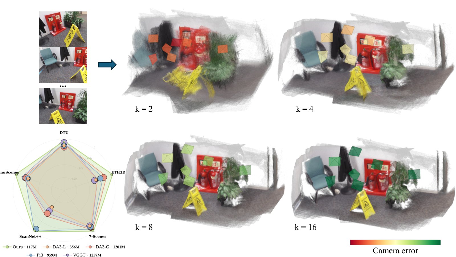
The averages are the paper's strongest evidence, and I recomputed them from Tables 1 and 2. Déjà View's mean inlier ratio is 80.3 (Pi3 77.4, VGGT-Ω 74.8) and its mean AUC@30 is 91.8 (VGGT-Ω 90.7, Pi3 88.6). The paper does not put the AUC@3 average in Table 3. I computed it: 57.2 for Déjà View against 47.0 for VGGT-Ω, 45.2 for Pi3 and 39.5 for VGGT. That ten-point lead on precise pose is the largest margin in any of the averages, and the paper undersells it by leaving it out of the summary table.
Cell by cell, the picture is more mixed. Counting all eight comparison models, including VGGT-Ω, which the paper marks as concurrent work:
- Pointmaps (Table 1). Déjà View is best on one of ten cells (DTU Rel. L2, a four-way tie at 0.009). It is second on eight. Pi3 leads indoor (7-Scenes, ScanNet++) and DTU inlier ratio; VGGT-Ω leads both outdoor sets (ETH3D, nuScenes).
- Pose (Table 2). Best on five of ten cells (ETH3D AUC@3, ScanNet++ both, nuScenes AUC@3, a tie on ETH3D AUC@30), second on four, third on one (7-Scenes AUC@3, 13.9 against VGGT-Ω's 21.3). The paper's caption, "first or second on nine of ten cells", checks out.
- VGGT still owns DTU pose. 96.5 AUC@3 against Déjà View's 83.2, with ten times the parameters.
Drop VGGT-Ω and Déjà View is best on most cells. Keep it and the summary is: best on average, rarely best on a single benchmark, never far from the best. For a model a tenth the size that is a good result, not a sweep.
Shared beats untied, at a smaller scale
The most interesting claim in the paper is not about size. Table 4 trains four variants for 100K iterations on the same data, from 16 independent blocks to the full gated, shared block:
| Variant | Rel. L2 | IR | AUC@3 | AUC@30 |
|---|---|---|---|---|
| Decoupled (16 blocks, no gates) | 0.056 | 61.1 | 23.0 | 82.0 |
| Shared | 0.045 | 66.4 | 30.2 | 84.8 |
| Shared + residual gates | 0.042 | 67.0 | 31.5 | 85.9 |
| Shared + state gate (full) | 0.040 | 69.2 | 33.3 | 86.9 |
Sharing alone beats the decoupled model on every metric, with 16 times fewer parameters in the loop and identical FLOPs. If this holds at full training, the case is that iteration with shared weights is a better inductive bias for multi-view geometry than depth with unique ones: the same refinement, applied again, generalises better than sixteen specialists.
I'd hold that loosely for now. These are half-length runs (100K iterations against the final 200K), and the absolute numbers are far from the released model's: inlier ratio 69 here against 80.3 in Table 1, AUC@3 33 against 57. A decoupled model at three times the parameters may simply train slower and catch up given the full schedule. The paper doesn't run it to the end, and that's the experiment I'd want before calling it an inductive-bias result.
What the loop learns to do
Two of the paper's analyses say something about what happens inside the loop.
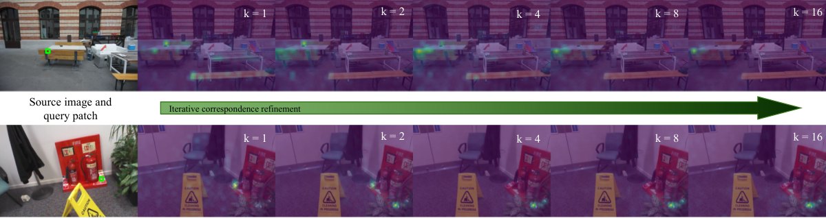
Appendix C reads the global attention weights from one query patch onto another view at each iteration. At the attention is diffuse; by it sits on the corresponding patch. Nothing in the loss asks for correspondences. The loop rediscovers feature matching because it needs matches to place cameras, and it does it iteratively, which is how SfM matching plus bundle adjustment works too.
The second analysis is Figure 3's "directional refinement". The state does not converge to a fixed point: its norm drops for the first few steps, then grows steadily through step 16. But its direction converges. Cosine similarity to the final state rises to 1, and the relative size of each update falls about fivefold. Each decoder starts with a LayerNorm, which throws away the norm, so from the decoder's point of view the state does converge.
That growing norm is also the failure mode. Push past the trained 16 and a few channels keep growing.
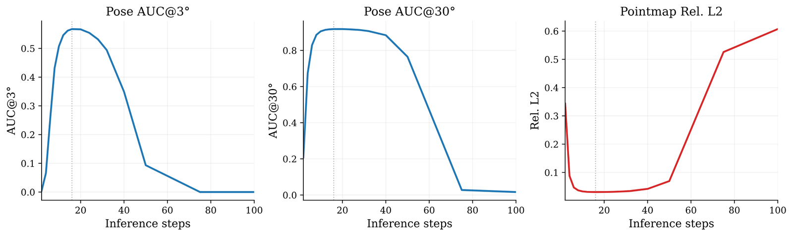
AUC@3 peaks at the trained budget and falls; AUC@30 and Rel. L2 hold to about 30 steps and then collapse. So the dial runs from 8 to 16. More compute past 16 buys nothing, and past 30 it breaks the model. This is the gap Solv3R set out to close: remove the time conditioning, inject the input at every call, and the block becomes a solver you can keep calling. Compare it with LiFT, a looped DiT that does keep improving past its training loops because each loop has an explicit regression target.
A second scene
Textured, static, overlapping views: the input these models like. The paper lists dynamic scenes as unsupported. For 360-degree walks through buildings under construction, with bare concrete walls and people crossing the frame, the indoor 7-Scenes and ScanNet++ numbers are the closest proxy, and there Pi3 still has the better pointmaps.
Where it stops
- The dial has two ends. Below 8 steps is untrained; past 16 the state drifts and past about 30 it collapses (Appendix D). Inside the range, re-grid; don't early-exit.
- Variable costs a little. Table 5: training with random matches a model trained at fixed to within about 2% at 16 steps, and a fixed model to within about 3% at 12. Flexibility is not free, just cheap.
- Compute is still quadratic in views. One block, sixteen times, is still sixteen global attention passes over every token. Long sequences need chunking or a streaming design, as with every model in its table.
- The weights are non-commercial. The code is Apache-2.0 (with VGGT-licensed files); the checkpoint is under NVIDIA's research-only licence.
- Two defaults. The quickstart runs 12 steps, the evaluation 16.
Official implementation of Déjà View: Looping Transformers for Multi-View 3D Reconstruction
- license
- custom
- branch
- main
- forks
- 27
- open issues
- 6
- source
- 1.4 MB
- commit date
- 2026-09-25
GitHub REST API, 2026-11-12 — branch, commit, commitDate, createdAt, description, forks, languages, license, openIssues, pushedAt, stars
- task
- image-to-3d
- library
- dvlt
- license
- other
- safetensors
- 1 shard
- largest file
- 468.4 MB
- files
- 5
- downloads
- 499
- likes
- 58
repo last modified 2026-05-30
Fewer parameters, not fewer FLOPs
I buy the parameter argument completely. A 14.5-million-parameter block, applied sixteen times on top of a DINOv2 ViT-B encoder (fine-tuned at a tenth of the learning rate), gets the best average accuracy on these five benchmarks against models eight to ten times its size. That says a lot of what a billion-parameter reconstructor stores is the same refinement, written out again with different weights.
I'd be more careful with the compute framing. The FLOPs are about half of VGGT's and Pi3's, and about the same as DA3-L's, because the cost of a reconstruction transformer is global attention depth times width times tokens squared, and looping does not change that equation. Where the paper's numbers show a real compute dial is pose precision: AUC@3 moves 14 points between 8 and 16 loops. If you need cameras for a splat or a survey, run 16. If you need a quick point cloud, run 8, and run it on an 8-step grid rather than stopping early.
The open question is whether shared weights beat untied ones at full training. If they do, the next billion-parameter reconstructor should probably be a hundred-million-parameter one with more loops.
How I checked. I ran: a safetensors-header parameter count (40,920-byte range request), the gate MLPs evaluated in NumPy from about 1.3 MB of range-fetched weights, a FLOP model of the forward pass, and the averages and ranks over Tables 1 and 2. I read Figure 8's values from its SVG path coordinates. I did not run the model or any of the repository's code, so every accuracy number is the paper's.