2026-11-09 · 36 min · 3d · slam · looped-transformers · vision-transformers · point-cloud · benchmarks
Why read this
Essentialtop 10%Solv3R's stationary looped block run from the released weights on CPU: convergence, ablations, continuation and 8-view block solves measured on real photos.
- Analysis found nowhere else
- Interactive explanations
- Runs on a consumer GPU
3D & spatialMixed licencesResearch paper
How this was scored
- Is it new?
- 2 of 3: A real new idea, method or capability
- Can I trust it?
- 2 of 3: Measures key facts from files, code or configs
- Can I run it?
- 2 of 3: Open code or weights with real limits
- Will I understand it?
- 3 of 3: Mechanism carried by interactives built from real code or data
- Can I act on it?
- 2 of 3: A concrete recipe, numbers or comparison
- Will it last?
- 2 of 3: A reference for a year or more
- Does it affect many?
- 1 of 3: A specialist community
- Only here?
- 3 of 3: The only place this analysis exists
Score 76 of 100, ranked 52 of 701 rated articles. Each question is answered 0–3 by hand, and a 3 is rare. How articles are scored
Every feed-forward reconstruction model I use at work has the same awkward moment. You reconstruct 40 photos, someone walks back in with 12 more, and the only honest option is to run all 52 again. Classical structure-from-motion never had that problem: it registers the new images against the map it already has and runs a few more rounds of bundle adjustment. The map is a state, and the optimiser picks up from it.
Solv3R (Jeong-gi Kwak, Andrea Tagliasacchi, Sho Kagami, Yuki Ono, Kwang Moo Yi; UBC, SFU, Wayve, Toronto, Sony) asks whether a geometric foundation model can behave like that optimiser. Its answer is a looped Transformer whose one shared block is trained to act as the iteration of a solver: the same update every call, no idea which call it is on, and a solved state that further calls leave alone. Tagliasacchi announced it as turning "a looped Transformer into a reusable learned geometric solver"; Kwang Moo Yi followed with the line that made me look closer: "Reconstruct full scenes by just solving 8 views at a time. <1.5GB VRAM is required to solve 128 photos. Basically, block coordinate descent." Code and weights landed on 5 November.
This is the second pass at this article. The first one could only read the checkpoint and time a block with random weights. This one runs the real thing: I wrote my own inference path from the released code, loaded the released weights into it, and put the repo's sample drone photos through the solver on a CPU. That turns most of the paper's solver claims from "reported" into things I could watch happen, and it found two places where the release behaves differently from what a reader would assume.
Why a feed-forward model cannot just continue
VGGT, π³ and Depth Anything 3 push a set of image tokens through a stack of different layers. Layer 7's output is only meaningful as layer 8's input. The tokens at depth 12 are "a scene, twelve layers into being solved", and there is no layer that accepts a mix of tokens at depth 24 (the old views, finished) and depth 0 (the new views, just encoded). So adding views means restarting.
Streaming models such as CUT3R dodge this with a recurrent memory, but they only take frames in order. A pile of extra photos from the other side of the building is not a video.
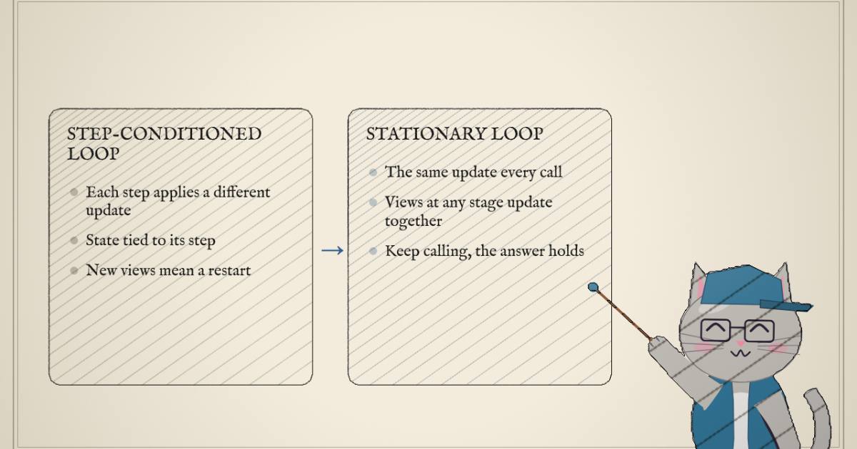
DéjàView, the model Solv3R starts from, already shares one Transformer block across 16 refinement steps. Sharing weights looks like it should fix the depth problem. The paper's point is that it does not, because DéjàView conditions each update on the step index:
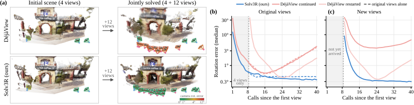
The block applies a different transformation at step 3 than at step 14, so a state is still tied to the step that produced it. Run it past step 16 and it is outside anything it was trained on; hand it views at mixed steps and no single fits them all. Figure 8 shows what that costs: DéjàView's error on the original views climbs again once new views join, while Solv3R's keeps falling.
The solver it imitates: Jacobi
The paper's running example is the oldest iterative solver there is. To solve , Jacobi applies the same update every iteration, , and does not know . When it converges you get three properties for free:
- P1, stability. The solution is a fixed point. More calls leave it alone.
- P2, correction. Knock the state off the solution and the same calls bring it back.
- P3, continuation. Add unknowns and equations, start the old unknowns at their solved values and the new ones at a guess, and keep iterating. Values that have had different numbers of iterations are updated together, because never asks how a value got there.
Map that onto reconstruction: the images are the constraints, each view's token state is the current estimate, the decoded cameras and depths are the solution. A learned multi-view solver should have all three properties. DéjàView has none of them by construction.
What Solv3R changes
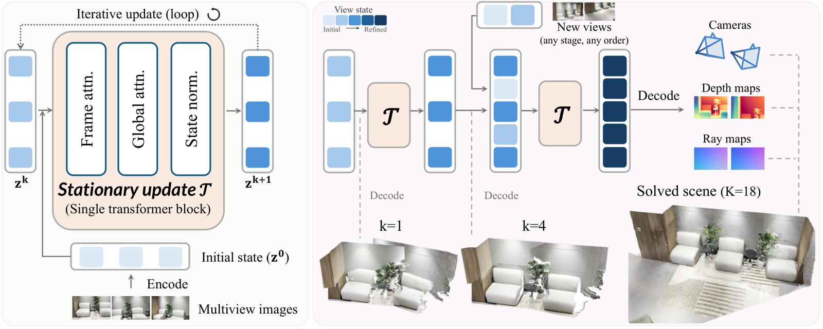
The update becomes
with one Transformer block (frame attention within each view, then global attention across all of them) shared by every call. Three changes to DéjàView make it stationary and keep it from drifting:
- Constant gates. DéjàView scales each sub-block's channels with gates computed from . Solv3R replaces them with learned constant vectors, initialised to the average of DéjàView's gates over its 16 steps.
- Initial-state injection. The encoded images are added back at every call through a zero-initialised projection, the way Jacobi reads and every iteration. Without it, an error in the state has nothing to be corrected against.
- One RMS rescale. After each call the whole state is scaled by a single factor to a fixed root-mean-square norm , so its magnitude cannot creep over 64 calls. One factor for all views keeps their relative scale.
One call, term by term
The supplementary material writes the call as (reported)
and the released code fills in every symbol. Take eight of the repo's park photos, 504 x 336 pixels each.
-
The state has shape . Each view is 869 tokens: one camera token, four register tokens and 36 x 24 = 864 patch tokens of 14 x 14 pixels. View 0 gets a different learned camera token from the others, and that is the whole mechanism that fixes the world frame to the first image.
-
The start is the DINOv2 ViT-B/14 encoding of each image (an affine-free LayerNorm on the patch features) with the camera and register tokens prepended. The solve starts at :
start()is a copy. -
The injection : is through a LayerNorm with no affine parameters, so every token enters at unit RMS; is a 768 x 768 linear layer with a bias. In the checkpoint its largest singular value is 0.319 and its Frobenius norm 1.86 (measured), so for a typical unit-RMS token it adds a vector of RMS around , about 8% of the state's 0.85 (reasoned). A quiet term, which is why the ablation below is surprising.
-
The block is two pre-norm sub-blocks. Each one computes, with LayerScale vectors and the constant gates ,
The first sub-block attends within each view (869 tokens, with 2D rotary positions on the patch grid); the second reshapes the state to one sequence of tokens and attends across all of them, with no positional encoding. Both use 12 heads of 64, QK-LayerNorm and a 3,072-wide MLP.
-
The rescale divides by one scalar, the RMS over all values, and multiplies by .
The third gate, , is the one I had not noticed in the paper. The code calls it the "output carry": it multiplies the whole residual stream, not an update. In the checkpoint every one of its channels is positive, between 0.20 and 1.04 in the frame sub-block and 0.25 and 1.01 in the global one, with means of 0.739 and 0.780 (measured). So each call shrinks the state channel by channel, to roughly 0.74 x 0.78 ≈ 0.58 of its size on average, adds the two updates, and lets the rescale bring the total back to 0.85 (reasoned). That is a contraction with a learned per-channel rate, which is what you would design on purpose if you wanted a fixed-point iteration to forget its starting point. The two update gates are less tidy: means 0.68 to 0.87, about one channel in seven negative, extremes from -1.08 to 2.48.
The released solv3r/network/block.py is short enough to read in one sitting,
and it is exactly this:
# solv3r/network/block.py (abridged)
def _frame(self, z, x0, pos):
    return self.frame_attn(z + self.inj(self.inj_norm(x0)), self.g_frame, pos)

def forward(self, z, x0, pos):
    S, P, C = z.shape
    y = self._frame(z, x0, pos)                                   # within each view
    y = self.global_attn(y.reshape(1, S * P, C), self.g_global)   # across all views
    rms = y.float().pow(2).mean((1, 2), keepdim=True).clamp_min(1e-12).sqrt()
    return self._rescale(y, rms).reshape(S, P, C)                 # one scale for the whole state
No argument carries a step. model.solve(ctx, calls=16) is a plain for
loop over that call, and model.add_views(z, ctx, images) concatenates the
new views' encodings onto the solved state, which is P3 as an API. Cameras come
out of the state through the ray head: its two-layer, 384-wide Transformer runs
on each view's tokens, and its output at the camera token goes through a small
MLP to a 9-vector: translation, a unit quaternion and two fields of view.
What the checkpoint says
I read the safetensors header of jgkwak/solv3r and pulled the small tensors
that pin the design down (measured):
| Part | Parameters | Trained in Solv3R? |
|---|---|---|
| DINOv2 ViT-B/14 encoder | 86.58M | frozen, from DéjàView |
| Solver block (frame + global) | 14.18M | yes |
| Injection projection | 0.59M | yes |
| Depth, ray and camera heads | 16.00M | frozen |
| Gates, tokens, RMS target | 0.01M | gates yes |
| Total | 117.36M | 14.78M trained (12.6%) |
All 117,360,839 values are fp32, which is the 469,484,684-byte file and the
"only 500mb weights" one early user on X was pleased about. The paper is
explicit that only the shared block, the gates and are trained; the header
agrees, with the encoder and heads carrying DéjàView's names
(base.patch_embed_encoder, base.depth_decoder) unchanged.
One detail the paper does not mention: the target_rms buffer holds four
numbers, 1.0045, 0.9783, 0.8501 and 0.8523, and the block reads only the last
(measured). The paper says is "the RMS of the final DéjàView state,
measured once before training ()". My guess is that the
other three are the same measurement at other points of DéjàView's stack or
schedule, left in the buffer; they do nothing at inference (reasoned).
What the code does that the paper does not say
Reading the release against the paper turns up five things that matter if you run it (measured, from the code):
- Precision.
autocast()is bf16 on CUDA and a no-op elsewhere, so every reported number is bf16 and everything on a CPU is fp32. My runs are fp32. - Which cameras.
decode()returns both the camera head's pose and dense rays;cameras_from_raysfits cameras to the rays and its docstring calls that "the benchmark protocol". The quick-start uses the camera head. I used the camera head, which is the cheaper path and needs no dense decoder. - The stopping rule.
examples/offline.py --adaptive 0.02checks the relative update from call 4 on and gives up at--max-calls 64. - The cache's scale. A cached call is exact for keys and values but not for the RMS rescale; more on that below, with a measurement.
- The 8-at-a-time mode. Not in the release. The README's to-do list still has "Release solver property examples" unticked.
How you train an operator to be a solver
Stationarity is a property of the architecture. Convergence is not; it has to be trained. The recipe (reported, from the appendix) is built to put the block in front of states it would meet in use:
- Windows. Each training window has 4 to 16, 24 to 32, or 48 to 64 views, drawn with probabilities 0.4, 0.3 and 0.3.
- Random depth. From the block runs a uniformly random 16 to 40 calls without gradients, then 8 calls with gradients, supervised only at the last one. Varying where supervision lands trains the block to give good geometry anywhere from call 24 to call 48, and to keep it there (P1).
- Perturbations. With probability 0.15 the state is perturbed before the gradient calls: Gaussian noise with standard deviation times the state's RMS, uniform in , or a reset of up to half the views back to . Noise teaches correction (P2); partial resets are what adding views looks like (P3).
- Losses. . The geometric term is L1 on ray directions and scale-aligned ray origins, geodesic losses on relative rotations and translation directions, a scale-aligned log-L1 depth loss (weight 0.5), a depth-gradient term where depth is dense, and two scale-consistency terms (weight 1.5 each) that tie every view's depth scale and camera centres to the window's. The distillation term applies the same ray, depth and camera losses against DéjàView's 16-step output, to keep its priors.
- Optimisation. AdamW, weight decay 0.01, learning rate 2e-5 for the block and and 2e-4 for the gates, an EMA of the weights with decay 0.999. About 70k iterations at batch 8 with growing windows, then 20k at batch 32 with the full recipe, on a 24-dataset mix led by ScanNet++ (10.8%), Infinigen (9.1%) and DL3DV (8.2%). A week on 8 H100s.
The paper compares it to denoising training and to Diffusion Forcing, and the comparison fits: the block learns from corrupted states it would otherwise never visit.
A solver you can poke
To see what P1 to P3 buy without a GPU, here is the paper's Jacobi analogy made concrete. Forty cameras sit on a ring; any two within eight places of each other share a noisy relative-offset measurement; camera 0 is the reference and fixes the world frame, as Solv3R's reference camera token does for view 0. One call is one Jacobi sweep. The stopping line is the paper's rule: stop when the relative state update falls below .
Running the same code under Node gives the numbers (measured, on the toy):
- P1. With 20 views, error falls from 0.524 to 0.0145 by call 16 and 0.0047 by call 200, and it never climbs back. Calling a solved ring changes nothing.
- P2. A perturbation that puts the error at 0.282 is undone by the same calls. The relative update drops under after 3 calls.
- P3. Solve 20 views, add 20 more from their starting guesses, and the 40 reach 1.1x their error floor in 14 calls; restarting all 40 from scratch takes 18.
- The stopping rule is a heuristic. In the toy, fires at call 4, when the error is still more than four times the floor: a slow, smooth error mode moves the state very little per call. The paper chose by measuring it on real windows, which is the only way to choose it.
The toy is linear and its properties are guaranteed by algebra. Solv3R's are trained into a nonlinear block, so they hold where training put them. The next three sections check them on the trained block itself.
Running the released block on real photos
The setup (measured): 8 of the 39 park photos, evenly spaced through the
flight (DJI_0737 to DJI_0777), encoded in 11.9 s, then 64 calls of the
solver at a median 2.36 s a call on 2 CPU threads, peak resident memory 1.43 GB
for the whole process. After each call I record and, at a set of calls,
decode the cameras. The reference is the block's own answer at call 64: the
widget's table gives the mean disagreement between that and the cameras at
earlier calls, as the angle between relative rotations over all 28 pairs of
views, so the world frame does not enter.
What the trace shows, with the released block as is:
- It settles where the paper says. falls from 0.786 at call 1 to 0.116 at call 8 and 0.0196 at call 16, the first call under . Sixteen photos of the same flight cross at call 17. The paper's 144 converging windows stop after 13 to 32 calls, 17.5 on average (reported); my two windows at 16 and 17 sit right in that range.
- The stopping rule stops at the right time here. At call 16 the cameras are within 0.14° of where they are at call 64 (mean; 0.32° for the worst pair). At call 4 they are still 2.7° away, and at call 8, 1.1°. Unlike my toy, where the rule fires early, on this trained block it fires once the cameras have stopped moving in any way that matters for a drone survey.
- P1 holds, with a floor. From call 16 to 64 the cameras drift another 0.14° in total, smoothly (0.13° from the final answer at call 24, 0.08° at 32, 0.03° at 48). But does not go to zero: it levels off at about 0.005 from call 50 on. The state keeps moving half a percent per call while the decoded cameras sit still. A trained operator has an approximate fixed point, not an exact one, and the motion that remains is in directions the camera head mostly ignores (reasoned; I did not decode depth to check whether the depth maps also hold still).
- The cameras are self-consistent. Nothing tells the model the photos came from one camera, and it worked that out: the decoded fields of view of the 8 views span 54.97° to 55.23° vertically and 75.80° to 76.23° horizontally. I cannot check the absolute value, because the sample photos carry no EXIF.
P2 on the real block (measured). I took the call-64 state, added Gaussian noise at 0.25, 0.5 and 1.0 times its RMS, and kept calling. The noise moved the cameras 0.41°, 0.85° and 1.93° off the solved answer. Sixteen calls later they were 0.040°, 0.138° and 0.236° off: back by a factor of 6 to 10 in every case, with at 0.008 and 0.012 for the two smaller perturbations and 0.021 for the largest, still settling. Recovery is not monotone, though: at the smallest noise the error dipped to 0.25° after one call, rose to 0.35° at call 4, then fell. That is a damped wobble, the signature of a contraction whose slowest mode is not a straight line home. The paper perturbs at call 8 with one and two times the state RMS and reports recovery from every one; my largest perturbation matches its smallest, and recovers.
Taking the three changes back out
The paper argues that injection, the RMS rescale and constant gates each earn their place. Its Table 4 (reported) retrains each ablation for 3k steps and reports pose AUC@5 at 16, 128 and 1,024 calls, and the rotation error after new views join:
| Variant (3k fine-tuning steps) | AUC@5, 16 calls | 128 | 1,024 | Join error (°) |
|---|---|---|---|---|
| DéjàView as released | 76.5 | 0.0 | 0.0 | 1.80 |
| Solv3R at 3k steps | 72.5 | 70.8 | 65.4 | 0.62 |
| step-conditioned gates, planned for 16 | 71.5 | 52.1 | 23.5 | 0.81 |
| no input injection | 71.6 | 33.1 | 0.0 | 0.64 |
| no state normalisation | 74.3 | 70.5 | 0.0 | 0.59 |
| no random-depth pre-calls | 73.1 | 3.4 | 0.0 | 4.37 |
| no perturbation training | 71.0 | 69.1 | 61.7 | 4.24 |
| Solv3R, final | 77.2 | 79.1 | 78.8 | 0.54 |
At 16 calls every variant looks fine, within about 6 points of the others. The table's lesson is that a fixed-budget benchmark cannot see any of this: the differences only show at 128 and 1,024 calls, or when views join.
I ran a cheaper, harsher version on the released checkpoint (measured, the widget's other buttons): take one component out at inference from a block that was trained with it, and run the same 8 views for 64 calls. This answers a different question from Table 4: not "could you train without it" but "what is it doing in this checkpoint". Three distinct failures:
- Without the injection the solve looks healthy for a while. falls to 0.024 at call 30, never quite reaching , and the cameras are 2.3° from the released answer at call 16. Then it comes apart: climbs back to 0.12, and the cameras drift to 5.8° off by call 32 and 15.2° by call 64. That 8% term is what keeps the state tied to the images. Without it, the block iterates on its own output and wanders, which is the paper's "errors in the state could accumulate over calls" made visible.
- Without the rescale nothing settles at all. The carry gates shrink the state every call, its RMS falls from 0.85 to about 0.54 and stays there, and from call 5 on stays between 0.35 and 0.73: most calls rewrite half the state. The cameras jump around between 2.3° and 6.1° from the released answer. The block has learned to work at one magnitude and is lost at another.
- With the gates set to 1 (roughly what removing them would mean, since they were trained around means of 0.68 to 0.87) the solve converges, slowly, to the wrong place. is still 0.022 at call 63, and the cameras sit 6.5° to 8.5° from the released answer from call 4 to call 64 without moving towards it. A stable fixed point, consistently wrong.
The three failure modes line up with the paper's retrained ones: no injection and no normalisation both collapse at long horizons there too. What the inference-time version adds is the shape of each failure: drift, thrash, and a confident wrong answer.
The evidence that the block behaves like a solver
The paper's own evidence, at scale (reported, from Section 4 and the appendix):
- Stopping. Over 148 eight-view windows (66 DTU, 37 ETH3D, 45 ScanNet++), 144 meet within 64 calls, after 13 to 32 calls (17.5 on average), and 143 of those 144 have camera rotation error under 5°. Harder windows take more calls.
- Stability past the schedule. DéjàView, trained for 16 steps, loses accuracy when run longer. Solv3R's accuracy holds to call 64. The appendix checks the inside too: the three global-attention heads that best find cross-view correspondences at call 16 still do at call 64, with an attention map similarity above 0.96; DéjàView's same heads fall below 3% correspondence accuracy by call 64.
- Mixed progress. Initialise each view from a random stage between 0 and 16 calls and independent trials agree on camera rotations to 0.08° on average.
- Continuation beats restarting. Inserting 64 views 8 at a time, continuing with 8 calls per insertion reaches an AUC@10 of 92.2; re-solving from scratch with 8 calls reaches 84.8 and needs 16 calls per insertion to reach 91.8. Insertion order (capture, reverse, random) moves the result by at most about two points.
Does accuracy suffer?
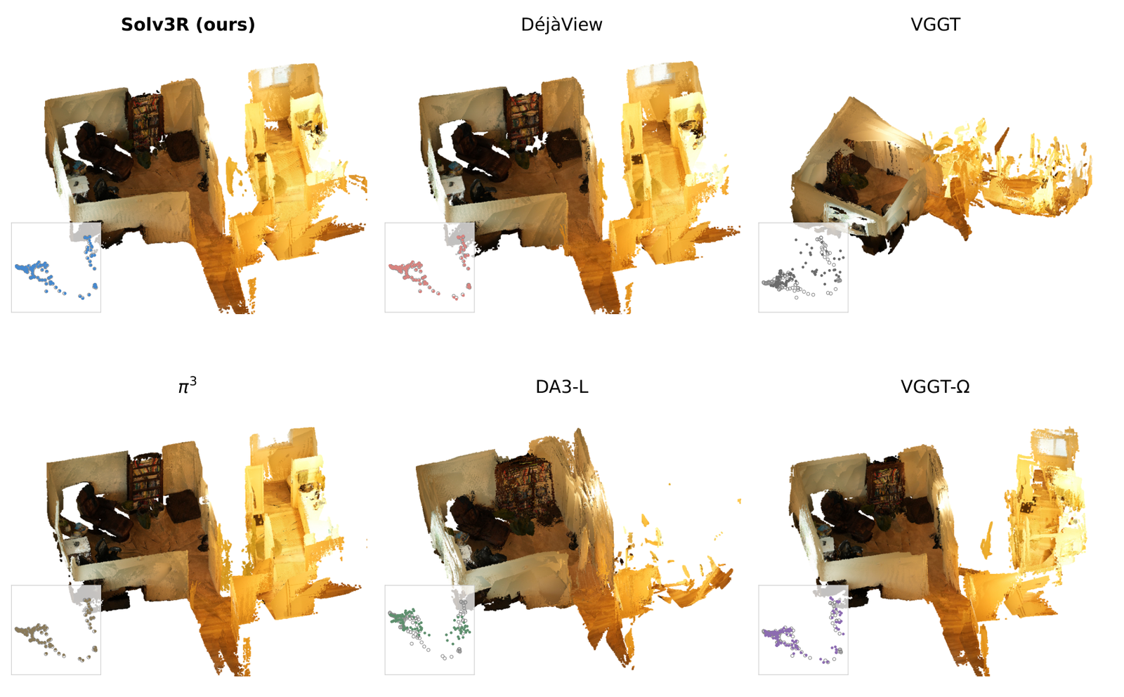
Not measurably against its own parent, which is the bar that matters for a fine-tune. The offline benchmark (reported, camera pose AUC@3, higher is better; TFLOPs for 24 views):
| Model | Params | TFLOPs | DTU | ETH3D | 7-Scenes | ScanNet++ | nuScenes |
|---|---|---|---|---|---|---|---|
| VGGT | 1.26B | 190.0 | 96.5 | 35.4 | 11.1 | 15.1 | 39.2 |
| VGGT-Ω | 1.14B | 99.8 | 77.4 | 64.1 | 21.3 | 29.9 | 42.4 |
| π³ | 959M | 153.8 | 70.2 | 43.2 | 11.3 | 76.5 | 24.8 |
| DA3-L | 411M | 71.4 | 79.4 | 42.0 | 11.4 | 7.0 | 10.9 |
| DéjàView, 16 steps | 117M | 75.9 | 83.3 | 66.0 | 13.9 | 79.5 | 43.4 |
| Solv3R, 16 calls | 117M | 76.5 | 84.5 | 65.4 | 13.8 | 80.7 | 41.5 |
| Solv3R, adaptive | 117M | 91.3 | 85.5 | 70.4 | 14.2 | 81.2 | 41.5 |
Read it plainly. At 16 calls Solv3R is DéjàView within a point or two either way, which is what a fine-tune that adds properties without losing accuracy looks like. The adaptive stop costs 3 to 4 extra calls on average and buys the best ETH3D and ScanNet++ numbers in the table. It does not win everywhere: VGGT owns DTU at AUC@3 and VGGT-Ω owns 7-Scenes. For a model a tenth of VGGT's size, that is a strong showing, but "state of the art" would overstate it. On two large aerial scenes from Mill19, with 96 images in one window, Solv3R has the best AUC@3 of the six methods (48.9 on Rubble, 22.5 on Building).
One cache, every call
The property I find most useful is a side effect of P1. If a map view is solved and held fixed, its keys and values in the global attention depend only on its own state. In a stationary block that state does not change, and neither does the block, so one cache is valid at every call. DéjàView needs a cache per step, and a stacked model like VGGT needs one per global layer.
That claim can be checked with nothing but shapes. A view's tokens are its patches plus a camera token and four registers; 7-Scenes frames are 640 x 480, which Solv3R resizes to 504 x 378 (36 x 27 patches) and VGGT to 518 x 392 (37 x 28):
977 tokens x 768 wide x 2 (K and V) x 2 bytes x 1 layer is 2.86 MiB. Sixteen step-specific copies make DéjàView's 45.8. VGGT's 24 global layers at width 1024 make 97.6. All three match the paper's Table 2 to the digit (measured arithmetic). The 16x saving is a counting fact about stationarity, not a compression trick.
What the small cache buys, in map-based relocalization (reported; queries attend to cached map views and only the query is refined):
| Model | Cache MB/view | ms/query | 7-Scenes within 5 cm, 5° | Cambridge within 25 cm, 2° |
|---|---|---|---|---|
| VGGT | 97.6 | 186 | 45.5% | 16.4% |
| π³ | 89.7 | 161 | 66.9% | 14.7% |
| DéjàView, one step's cache | 2.86 | 50 | 0.0% | 0.0% |
| Solv3R | 2.86 | 51 | 72.8% | 24.9% |

The DéjàView row is the control that makes the argument: give a step-conditioned model only one step's cache and it localises nothing.
How exact is the cache? (measured). The keys and values of a held view are
exact by construction. The RMS rescale is not: it needs the sum of squares of
every view's output, and cache() computes the held views' share by running
global attention among the held views only. The docstring says this is
"close to the full call when the reference view (view 0) is held". I checked
both cases on the 16-view state at call 16, splitting the views into a held
half and an updated half, and compared one cached call with the same rows of
the full joint call:
- View 0 held: the cached output differs from the joint call by 0.099% of its norm, while the call itself moves those views by 1.79%. About a twentieth of the update is error. Fine.
- View 0 in the updated half: the difference is 1.41%, against an update of 1.77%. The error is four fifths the size of the step. That is not "close to the full call"; it is a different call.
So the docstring is right about the case it names, and the streaming setup holds view 0 among its anchors, so streaming is in the good case. Anything else that holds views should keep view 0 in the held set, or recompute the scale.
Eight views at a time
Now Kwang Moo Yi's claim: solve 128 photos 8 at a time, under 1.5 GB of VRAM.
The authors' version is not in the release. The ballroom image of 128 photos
solved 8 random photos at a time links to a video, not to code, so how they
choose blocks, and whether the reference view rides along, is unpublished. The
pieces are in the API (Context.subset, model.cache, model.step_cached),
so I wrote the obvious version and ran it.
The memory claim is plausible from the sizes (reasoned). For 128 photos at 504 x 336 (869 tokens a view) the state and the encodings are 2 x 128 x 869 x 768 fp32 values, 652 MB. The weights are 469 MB in fp32. Together that is about 1.12 GB, leaving a few hundred MB for one 8-view call's activations in bf16. Under 1.5 GB is believable; a joint call on all 128 would not be close.
The compute side, on a shape-matched block (measured). Before I had the real weights running, I timed one call of a block with Solv3R's shapes and random weights, on 2 CPU threads in fp32:
One 8-view call took 1.94 s and one 64-view call 68.67 s, 35 times longer for 8 times the views, because global attention grows as the square of the tokens in the call. The real block, on a busier box, ran 8 views in 2.36 s and 16 in 6.57 s, about 20% over the shape-matched curve. A sweep that gives each of 128 views one call in blocks of 8 is 16 calls, about 31 s, against an extrapolated 4.3 minutes for a single joint call.
Does block-at-a-time reach the joint answer? (measured). This was the question the first version of this article could not answer. I took 16 park photos, solved them jointly for 48 calls as the reference, and reached the same 16-view solve three other ways:
- Restart: all 16 from their encodings, jointly.
- Continue: 8 photos (every other one, including view 0) solved for 16 calls; then the other 8 join from their encodings and all 16 keep going. P3, on real photos.
- Blocks of 8 with a cache: each sweep splits the 16 at random into two halves; the first half takes one call while attending to a cache built from the other half's current states, then the second half does the same against the first half's new states. Block Gauss-Seidel: every view gets one call per sweep, and no call carries more than 8 views' queries.
The numbers, as mean disagreement with the joint 48-call answer:
| Calls per view | 4 | 8 | 12 | 16 | 24 |
|---|---|---|---|---|---|
| restart, all 16 | 2.53° | 0.63° | 0.19° | 0.116° | 0.100° |
| 8 solved, 8 join | 1.45° | 0.27° | 0.13° | 0.099° | 0.097° |
| blocks of 8, cached | 2.82° | 0.50° | 0.20° | 0.116° | 0.097° |
Three things to read from it:
- Continuation pays, early. Eight calls after the join, the continued solve is 0.27° from the joint answer and the restart 0.63°. By call 16 the two are within 0.02° of each other. That is the paper's AUC@10 result (92.2 continued against 84.8 restarted at 8 calls) in miniature: the head start matters when you cannot afford many calls, and stops mattering when you can.
- Blocks with a cache converge to the joint fixed point. After 24 sweeps the block solve is 0.097° from the joint answer, the same as a 24-call joint restart (0.100°) and closer than the joint solve's own call 16 is to its call 48 (0.116°). In every sweep one of the two half-updates had view 0 in the updated half, the case where the cached scale is off by 1.4% per call; the cameras did not care. So Kwang Moo Yi's "basically, block coordinate descent" describes something that works, at least on 16 photos of one flight.
- Blocks without a cache do not. As a control, I solved the two halves separately, each on its own for 32 calls, the second half with its first photo promoted to reference view. Within the half that held view 0, relative rotations agree with the joint answer to 0.32°; within the other half, to 10.6° (19.2° for the worst pair). One sample, so not a rate; but the eight photos that did badly alone were fine inside the joint and the cached solves. What made the block solve work was the other views' keys and values, not the block size.
The cost result is the one I did not expect (measured). On 16 views a sweep of two cached half-updates took 11.0 s, against 6.6 s for one joint call. The reason is in the cache: in block coordinate descent the held views change every time a block is updated, so the cache is rebuilt every call (frame attention and a key/value projection for every held view), and the release's scale computation runs global attention among all the held views, which is the quadratic term again. Below some size the joint call is simply cheaper. At 128 photos in blocks of 8 the query side is 8 views against 128, so that attention grows linearly in the scene and the memory story holds; but the held-scale term has to go (keep a running sum of squares instead, the obvious fix, reasoned) before the compute story does too.
Streaming falls out, too
The same weights stream without streaming-specific training (reported). The default L8 setup keeps 8 anchor frames, 6 recent frames that keep refining, and up to 64 memory frames taken every 16th frame; anchors and memory are held fixed and enter every call through that one-layer cache. A new frame does not start from its bare encoding: it starts from its encoding plus the previous frame's solved offset, roughly , a warm start that makes sense only because a neighbouring frame's state means the same thing at any call. Every four frames, one extra call measures on the frozen views; above 0.02 they rejoin the solve and their cache is rebuilt, which is P2 used as a consistency check. Memory stops growing once the memory bank fills, after about 1,030 frames. On the long 2,000-frame TUM office sequence, offline VGGT runs out of an 80 GB H100 at 320 frames. The README's expected camera ATE for L8 is 0.157 on Sintel, 0.015 on TUM-dynamics and 0.077 on ScanNet. Pipelining also works because views at different stages are fine: the window can advance after every call, so a new frame's latency stays the same while throughput is 16x DéjàView's re-solve-per-frame (10x end to end). The DA3 streaming piece covers the other way to bound memory, with a keyframe bank around a frozen backbone.
Where it breaks, and what it costs
- Low overlap. The paper's one failure window has views 5 to 8 sharing little with views 1 to 4; Solv3R places the second group wrong within 16 calls and keeps it there to call 64. A solver converges to a fixed point. Nothing makes it the right one when the constraints are weak, which is true of bundle adjustment too, and which my gates-at-1 run showed from the other side: a stable, wrong fixed point looks like a converged solve to .
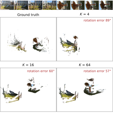
- The stopping rule cannot see a wrong answer. measures motion, not error. In my runs it fired at the right time on a good solve, and with at 0.022 instead of 0.02 it would have fired on the gates-at-1 solve too. Pair it with a check that does not come from the solver, such as reprojection error.
- Density. Inputs are resized so the long side is 504 px, and depth comes out at that resolution. "The density/quality is hurting" was the same early user's verdict. That is the price of a 117M model, not of the solver idea.
- Licences. The code is Apache-2.0. The weights are built on NVIDIA's DVLT and ship under the NVIDIA License: non-commercial, research and evaluation only. I would not build a product on them.
- CPU. It runs on CPU: my fp32 runs took 12 s to encode 8 photos and 2.4 s
per 8-view call, so a 16-call solve of 8 photos is under a minute, and peak
memory was 1.4 GB for 8 views and 2.1 GB for 16.
from_pretraineddefaults todevice="cuda", so passdevice="cpu".
What I could not check
- Accuracy. The park photos have no ground-truth poses, so all my camera numbers are agreement between solves of the same block. A solve can agree with itself and be wrong, as the gates-at-1 run shows. Every accuracy number in this article is the paper's.
- The released package. I ran my own re-implementation, not
pip install -e .. It loads every tensor it uses from the checkpoint by name, and its behaviour lands on the paper's (settling at 16 to 17 calls, consistent fields of view across views, recovery from noise), but I have no reference output to diff against, and a subtle bug of mine would show up as worse numbers, not as an error. - bf16. All reported numbers are bf16 on a GPU; mine are fp32. The 0.005 floor on may be different in bf16.
- Scale. Two windows of 8 and 16 photos from one drone flight, against the paper's 148 windows. My numbers say the mechanisms work on these photos; the paper's say how often.
- The dense heads. I did not port the depth and ray decoders, so nothing here checks depth or point maps.
Where it sits
The idea is not "loop a Transformer"; DéjàView did that, and the looped language models before it (what separates Ouro from Huginn, looped versus deep at matched compute). Nor is the fixed-point view new: deep equilibrium models and path-independent equilibrium models argued that an iterated block should converge to the same answer from any start, and the paper cites them. What Solv3R adds is a geometric reason to want that property and three cheap changes that get it from a pretrained step-conditioned model: constant gates, injection, one RMS scale. My two roundups of this year's feed-forward reconstruction work, the first and the second, were mostly about bolting classical machinery onto networks that cannot iterate. Solv3R puts the iteration inside the network.
Running it
From the README, on a machine that will run the package (mine would not, so everything measured above went through my own re-implementation):
git clone https://github.com/ubc-vision/solv3r.git && cd solv3r
pip install -e .
python examples/offline.py     --images examples/data/park --out outputs/offline --sky-mask
python examples/incremental.py --images examples/data/park --out outputs/incremental --initial 8 --group 4
python examples/streaming.py   --frames examples/data/desk --out outputs/streaming
--adaptive 0.02 turns on the stopping rule for offline solves, and
--config L4 or S4 picks a lighter streaming setting. The park sample is 39
drone photos at 504 x 336, the photos every measurement above used.
- license
- Apache-2.0
- branch
- main
- tests
- none found
- source
- 145.5 kB
- commit date
- 2026-11-06
by size of tracked source at this commit, file counts in brackets; docs, data and vendored trees excluded
local clone, 2026-11-10 at ef8da34 — branch, commit, commitDate, fileCount, hasTests, languages, license, licenseFile, shallow
shallow clone: counts describe the pinned tree, not the history
- task
- image-to-3d
- license
- other
- safetensors
- 1 shard
- largest file
- 469.5 MB
- files
- 4
- downloads
- 0
- likes
- 9
repo last modified 2026-11-05
What to take from it
Make the loop stationary, then train it to have a solver's properties. Everything practical follows from that one constraint, and on the released weights I could watch each piece work: a solve that stops at call 16 with its cameras already still, noise that the same calls remove, eight new photos that join a running solve and reach the joint answer faster than a restart, and half the scene updated at a time against a cache of the other half landing on the same answer as the whole. The two cautions are just as concrete. The cached call's scale is only right when view 0 is held, and a stable fixed point can be a wrong one. What I want next is the authors' 128-photo block example, run against ground truth.