2026-11-09 · 35 min · point-cloud · 3d · self-supervised · vision-transformers · lidar
Why read this
Notabletop 60%How a plain ViT over voxel patches and four leak-plugging changes push 3D self-supervised features past PTv3, with token counts and tokenizer norms measured.
- Original analysis
- A lasting reference
- A new technique
3D & spatialNothing to runResearch paper
How this was scored
- Is it new?
- 2 of 3: A real new idea, method or capability
- Can I trust it?
- 2 of 3: Measures key facts from files, code or configs
- Can I run it?
- 0 of 3: Closed, nothing to run
- Will I understand it?
- 2 of 3: Mechanism from first principles with figures
- Can I act on it?
- 2 of 3: A concrete recipe, numbers or comparison
- Will it last?
- 2 of 3: A reference for a year or more
- Does it affect many?
- 1 of 3: A specialist community
- Only here?
- 2 of 3: A teardown or measurement few others did
Score 60 of 100, ranked 396 of 701 rated articles. Each question is answered 0–3 by hand, and a 3 is rare. How articles are scored
Every 3D self-supervised model I have tried on a real scan has the same tell. Freeze the encoder, fit a linear head, and the chair legs come out the same colour as the table legs. They are both thin vertical cylinders. The features learned geometry, not objects. In 2D, a frozen DINOv2 with a linear head gets close to a supervised model. In 3D it has not.
VINO (Adrian Kruse, Kadir Yilmaz, Daan de Geus, Francis Engelmann and Bastian Leibe; RWTH Aachen, TU Eindhoven and USI Lugano; arXiv 4 November 2026) is a paper about why. Its authors posted it as "DINO for 3D/volumetric data". It takes Sonata, the current reference recipe for 3D self-distillation, and changes five things: the backbone, how the teacher sees the scene, where its targets come from, what the student sees when part of the scene is masked, and how 2D image features are distilled in. Each change is small. Together they move ScanNet200 linear probing from 28.3 to 40.4 mIoU on the paper's own ablation path.
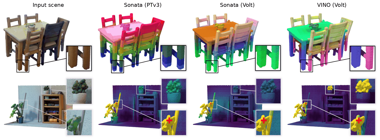
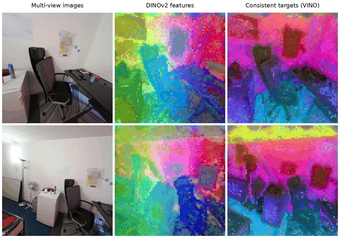
The figure's middle column is the useful control. Sonata's recipe on the new backbone looks like Sonata's recipe on the old one. Whatever VINO fixes, the backbone swap is not most of it, and the ablation table agrees.
What you can check today is limited. The VINO repository is a README: "Code and pretrained weights are coming soon." The backbone it builds on, Volt (same group, April 2026), is open under MIT. So I read the VINO paper and the Volt code, re-implemented Volt's tokenizer and encoder, and ran them on CPU on Pointcept's demo scenes. Volt's repository is a fork of Pointcept, so it also carries Sonata's released pre-training config and model, the baseline every one of VINO's fixes is aimed at. That let me hold the paper's description of Sonata against Sonata's code, and count what each backbone costs on the same voxels. Labels below: measured is a number I produced, reported is the paper's, reasoned is my inference.
- license
- MIT
- branch
- main
- tests
- 9 files
- source
- 4.5 MB
- commit date
- 2026-09-15
by size of tracked source at this commit, file counts in brackets; docs, data and vendored trees excluded
local clone, 2026-11-10 at 8dcd608 — branch, commit, commitDate, fileCount, hasTests, languages, license, licenseFile, shallow, testFileCount
shallow clone: counts describe the pinned tree, not the history
The backbone change: from a U-Net to a ViT
Sonata and almost every recent 3D self-supervised method (Concerto, Utonia, DOS, PointINS, LAM3C) use Point Transformer V3. PTv3 is hierarchical: it serialises points along space-filling curves, attends inside local windows, pools, and repeats at coarser resolutions, like a U-Net. Dense self-distillation on a hierarchy needs a feature at every point, so Sonata upsamples the outputs of several stages and concatenates them before the loss.
Volt does what ViT did to images. From the Volt code
(pointcept/models/volt/volt_base.py, commit 8dcd608):
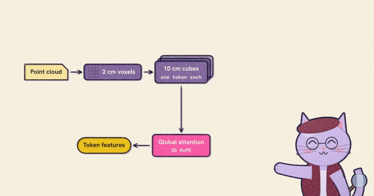
- Voxelise the cloud on a 2 cm grid indoors, 5 cm outdoors, one point per occupied voxel.
- Cut space into non-overlapping cubes of P x P x P voxels, P = 5. That is a 10 cm cube indoors and 25 cm outdoors.
- Each non-empty cube becomes one token: scatter its voxels' features into a
dense
[125, C]block, zero the empty slots, flatten, and apply onenn.Linear(125 * C, D). - Run a plain pre-norm Transformer over all tokens with full global attention (FlashAttention varlen, one sequence per scene) and 3D RoPE on the integer patch coordinates.
- A single transposed-convolution-like layer (a linear to
125 * D'and a gather) puts features back on the voxels.
No windows, no serialisation, no pooling. The interesting question for a ViT on 3D is how long the sequence gets, because attention is quadratic in it. Volt's paper says "on the order of 5,000 tokens" for a ScanNet scene. I counted.
Measured. Pointcept's sample1 is an indoor room, 273,530 points over
7.2 x 8.0 x 2.5 m. At 2 cm it has 187,899 occupied voxels. With P = 5 those
collapse to 12,092 tokens, about 240 times fewer attention pairs than one token
per voxel. The room is larger than a typical ScanNet scan, which is why it
lands above the 5,000 figure; VINO crops indoor views to at most 65,536
voxels during pre-training (reported). I cut that crop out of the room, the
65,536 voxels nearest its centre, and it makes 4,425 tokens (measured; an
earlier version of this article estimated about 4,200 by proportion).
The number I did not expect is the fill. A token has 125 slots and the room fills 15.5 of them on average, median 15. One token in three has ten or fewer occupied voxels. Surfaces are 2D, so a 10 cm cube cut through a wall holds one sheet of voxels, about 25 of 125, and a cube that clips the edge of a chair leg holds three. Outdoors it is starker: the LiDAR sweep at 5 cm gives 32,700 tokens with a median of 2 occupied voxels each, 3.1% fill. VINO caps outdoor crops at 6,000 tokens (reported). That sparsity is the reason two of VINO's four fixes exist, as we will see.
I also ran a forward pass. The sandbox would not execute the downloaded Volt
code, so I wrote the encoder again from the source: the same tokenizer, RoPE
cache (theta 100, frequency split 12/12/8), QK-norm attention blocks and
detokenizer, with PyTorch's scaled_dot_product_attention in place of
FlashAttention. Measured (PyTorch 2.14.1, 2 CPU threads, random weights,
fp32): Volt-S (384 wide, 12 blocks, 6 heads) has 23.68M parameters and takes
19.1 s for the 12,092-token room; Volt-B (768 wide, 12 heads) has 85.63M
parameters without its decoder and takes 42.1 s. Peak RSS was under 2 GB. The
85.6M matches the "Volt-B (85.7 M)" in VINO's tables, so the architecture the
paper describes is the one in the Volt repository. The CPU times say nothing
about GPU speed; the Volt paper reports Volt-B as twice as fast as PTv3-S on
A100 and H100 (reported).
A correction to the first version of this article, which gave 87.78M "with the
decoder". That figure used Volt-S's decoder width (up_mlp_dim=128). Volt-B's
configs set 256, and at 256 the decoder is 8.39M on its own (a 768-to-256
linear, two batch norms, and a 256-to-32,000 detokenizer), for 94.03M in all
(measured, counted from the code). VINO's Table 5 lists the supervised Volt-B
with decoder at 94.3M; the remaining 0.3M is the segmentation head and
whatever else that model carries, which I cannot see without its config.
Volt-B with shapes
Here is one forward pass with the tensor shapes the code produces, for the 65,536-voxel indoor crop (T = 4,425 tokens, measured) and Volt-B's widths:
| Step | Operation | Shape out | Parameters |
|---|---|---|---|
| Voxelise | 2 cm grid, one point per voxel, features = RGB + normal | [65536, 6] | 0 |
| Patchify | indices // 5, unique, scatter into slot x*25 + y*5 + z | [4425, 125, 6] | 0 |
| Tokenize | flatten, nn.Linear(750, 768) | [4425, 768] | 576,768 |
| RoPE | per-axis angles from integer patch coords, 12 + 12 + 8 frequencies | [4425, 32] complex | 0 |
| 12 blocks | pre-norm; QKV [4425, 3, 12, 64], LayerNorm on q and k, RoPE, attention over all 4,425; MLP 768 → 3,072 → 768 | [4425, 768] | 12 × 7,088,128 |
| Decoder | BN, GELU, Linear(768, 256), BN, GELU, Linear(256, 125 × 256), gather each voxel's slot | [65536, 256] | 8,390,912 |
The RoPE row is worth a second look. Each head is 64 wide, which is 32 complex pairs, and Volt gives 12 of them to x, 12 to y and 8 to z, with frequencies spaced geometrically between 1 and 1/100 (theta = 100, not the 10,000 of language models). Patch coordinates are integers in 10 cm steps; a cache is precomputed for 1,024 positions on x and y and 512 on z, so one sequence can span 102 m by 102 m by 51 m indoors, and two and a half times that at the outdoor 25 cm patch. There is no absolute position embedding anywhere: the only thing a token knows about where it is comes from these rotations, applied to q and k inside attention. That is what VINO's masked predictor relies on, as we will see. The site's RoPE explainer covers the 1D version.
What a plain ViT costs on voxels
"Simpler" and "cheaper" are different claims, and the Volt paper makes the second one with wall-clock numbers on GPUs I do not have. What I can count is work. I wrote a cost model for both backbones from their layer shapes and ran it on the same voxels: Sonata's PTv3-B encoder exactly as its pre-training config sets it (channels 48 to 512, depths 3/3/3/12/3, 1,024-point attention windows, a 3x3x3 submanifold convolution as positional encoding in every block, grid pooling by 2 between stages), against the Volt-B encoder. Two checks first. My parameter count for that PTv3-B config is 108.45M, which matches the 108.4M in VINO's tables. The convolution cost uses each voxel's real number of occupied neighbours, which I counted: 8.5 per voxel at stage 1 on the indoor crop, rising to 13.7 by stage 5 (measured). Sparse convolution only pays for the neighbours that exist.
Measured (forward GFLOPs, two times the multiply-adds, from shapes and neighbour counts, not a profiler):
| Input | PTv3-B encoder | Volt-B encoder | Ratio | Attention share in Volt |
|---|---|---|---|---|
| Indoor, 65,536-voxel crop (4,425 tokens) | 406 | 1,479 | 3.6x | 49% |
| Indoor, whole room (12,092 tokens) | 1,130 | 7,458 | 6.6x | 72% |
| Outdoor, crop near VINO's 6,000-token cap (6,188 tokens) | 527 | 2,470 | 4.7x | 57% |
| Outdoor, whole sweep (32,700 tokens) | 2,753 | 45,011 | 16.4x | 88% |
Three things come out of this.
Volt-B does more arithmetic, by 3.6x at the size it trains on. PTv3 is cheap because its widths are small where its point counts are large: 48 channels over 65,536 voxels at stage 1, and the 384- and 512-wide stages run on 1,776 and 427 points. Volt runs 768 channels on every token, every block. The Volt paper's "twice as fast as PTv3-S" (reported) is therefore not a FLOP claim. It is a claim about what a GPU does with dense matrix multiplies and FlashAttention, against gathers, scatters, hash lookups for the sparse convolution, four space-filling-curve sorts and padding to 1,024-point windows. I find that plausible (reasoned) and cannot check it here. It also compares against PTv3-S, not the PTv3-B in the self-supervised tables.
Volt does fewer attention pairs, not more. Summed over all blocks, PTv3-B scores 328M query-key pairs on the indoor crop and Volt-B 235M (measured). PTv3 has 24 blocks and pads every stage to whole windows of 1,024; Volt has 12 blocks over a sequence a fifteenth as long as stage 1. Quadratic attention over patches is cheaper than windowed attention over voxels at this scale. Volt's cost is the width, not the attention.
The crossover sits right at the training size. Per block, attention costs about 4T²D and the linear layers 24TD², so they are equal at T = 6D, which is 4,608 tokens for Volt-B (reasoned, from the shapes). The indoor training crop is 4,425 tokens and attention is 49% of the encoder; the outdoor cap of 6,000 tokens puts it at 57%. Run Volt-B on a whole LiDAR sweep, which you would do for inference if you did not tile, and attention is 88% of 45 TFLOPs. The cap VINO puts on outdoor crops is a compute decision as much as a data one, and whole-scene inference outdoors is where the quadratic term will bite (reasoned).
The table under the widget shows the other half of the trade. A 1,024-voxel z-order window at PTv3's first stage spans a median of 1.0 x 0.9 x 0.6 m indoors (measured); only at stage 4, after three poolings, does a window cover a room-sized 5 x 4 m. Volt's first block attends across the whole crop. Whether that global reach is what lets VINO tell a chair leg from a table leg, I cannot separate from the training changes: Table 1's architecture swap alone is +1.3.
Swapping the backbone alone, Sonata's recipe goes from 28.3 to 29.6 on ScanNet200 linear probing (reported, Table 1). A 1.3-point gain is real but modest. The bigger effect is downstream: with one flat sequence of tokens, every trick from 2D self-distillation (registers, cross-attention predictors, dropping masked tokens) applies without adapting it to a multi-stage pyramid.
The four leaks
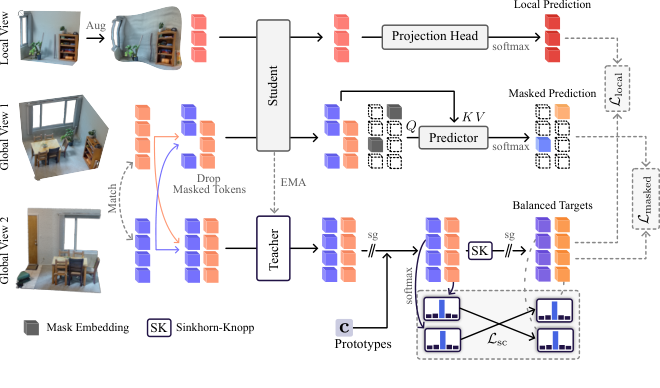
Self-distillation has two objectives. Local prediction: a student sees a small crop and must predict, at each token, what the teacher said about the same location in a big crop. Masked prediction: the student sees a big crop with blocks hidden and must predict the teacher's output at the hidden blocks. Both work when the only way to solve them is to understand the scene. VINO's argument is that, in 3D, each objective as Sonata built it has a shortcut.
Leak one: the teacher sees what the student sees
Sonata applies the same augmentation set to every view: elastic distortion, dropout and jitter on the teacher's global crops as well as on the student's local crops. The teacher's targets are then computed from warped geometry. VINO keeps the teacher's two global views clean (standard rotations, flips, scaling and coordinate jitter only) and puts the strong corruptions only on the student's four local views: three of elastic distortion, point dropout, colour jitter and chromatic translation indoors (reported). This alone is +2.4 mIoU (Table 2).

Leak two: the target head drifts toward the student
In DINO, the teacher's projection head is an exponential moving average of the student's. Once the two see different input distributions, that coupling makes the teacher's head track one adapted to corrupted inputs. VINO replaces it with a target head that belongs only to the teacher, borrowed from CAPI: 4,096 learned prototypes , cosine similarities to the teacher's token features , sharpened by a temperature and balanced with three Sinkhorn-Knopp iterations:
The prototypes cannot be trained by the student's loss without collapsing, so they get their own: for each pair of corresponding tokens in the two global views (nearest token centres, at most 2 tokens apart), the balanced assignment of one is the target for the other's softmax over prototypes, and vice versa. In the paper's notation (reported, Eq. 2):
Term by term: is the set of corresponding token pairs across the two clean global views; is token 's balanced Sinkhorn assignment from Eq. 1, held fixed (no gradient); is the plain softmax of token 's cosine similarities at temperature , which does carry gradient, but only into the prototypes , because the teacher encoder is stopped too. A prototype is pulled toward whatever direction makes two views of one surface land in the same cluster. Nothing in this loss sees the student. That swapped clustering loss updates only the prototypes. The student's head is a separate MLP trained with cross-entropy against .
Compare Sonata's head, from its code: an MLP 1,088 to 4,096 to 256, L2 normalisation, and 4,096 weight-normalised prototypes, the whole head copied into the teacher by EMA, with the teacher's temperature warming from 0.04 to 0.07 and the student's at 0.1 (measured, read from the config). The Sinkhorn step is the same three iterations in both. What changes is ownership: in Sonata the teacher's prototypes are an average of the student's; in VINO they belong to the teacher and are trained by a loss the student never touches. Reported: +1.5 mIoU (Table 2), and it is what makes leak three's fix possible, because masked prediction reuses the same targets.
Leak three: the mask keeps the shape
This is the change I find most convincing, and the one where 3D differs from 2D for a real reason. In an image every patch exists; masking a patch with a learned embedding hides its content and nothing else. In a sparse voxel grid, which tokens exist is itself the geometry. Sonata and other scene-level methods replace masked features with a mask embedding but leave the tokens where they are. The student then sees the exact outline of every masked region and can predict "table" from "flat slab at 75 cm" without looking at any context.
How much does that outline tell you? I measured it on the demo room with VINO's masking settings: 8-token blocks (80 cm) with 55% of blocks masked, the token label being the majority ScanNet-20 class of its voxels. For each masked token I built a lookup from its own geometry to a label, fitted on a random half of the masked tokens and scored on the other half, over 10 random masks.
| What the predictor sees about a masked token | Accuracy (measured) |
|---|---|
| nothing (most common class) | 29.7% |
| its height in the room | 57.2% |
| its occupied-neighbour pattern (in-plane and above/below counts) | 54.6% |
| height and neighbour pattern | 62.2% |
A two-key lookup table, with no learning and no context, gets 62% of masked tokens right in a room where guessing gets 30%. A Transformer with the whole masked outline available can do much better than a lookup table. That is the shortcut. The demo room has only ten classes present and 12,092 tokens, so treat these as an illustration of scale, not a benchmark.
VINO deletes masked tokens before the student encoder, as MAE does for images and Point-MAE does for objects. A small decoder of four cross-attention layers then places one query, a learned mask embedding, at each masked position and lets it attend to the encoded visible tokens with the same 3D RoPE. Queries do not attend to each other, so no query can see where the other masked tokens are. Reported (Table 11): cross-attention only 35.9, adding query-to-query attention 34.2, a full self-attention decoder 33.0.
My measurement also shows what is left (reasoned). Each query still carries its own position, and through RoPE its offset from the visible floor and walls. The height row above, 57%, is information VINO does not remove, and probably should not: knowing where you are is part of the context. What VINO removes is the neighbour pattern, the shape of the hole. Adding masked prediction this way is worth +2.8 mIoU (Table 3), the largest single step in the self-supervised stage.
Leak four: the tokenizer counts voxels
Volt's tokenizer is a weighted sum over a patch's occupied slots. A patch with 40 voxels sums 40 contributions; a patch with 3 sums 3. The paper traces high-norm token artifacts that survive register tokens to exactly this: early in training, before semantic features exist, the token's magnitude encodes how full its patch is, and the student can match the teacher on that. VINO divides the sum by the number of occupied voxels: an average.
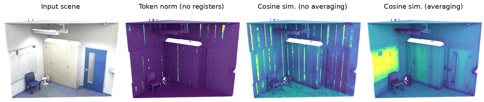
I wanted to see the effect in numbers, so I measured token norms at initialisation on the demo room, 12,092 tokens, Volt's init (truncated normal, standard deviation 0.02). There is a twist.
Measured. With Volt's tokenizer as built, every slot of the 125 has its own block of weights. At random init, the contributions of different voxels point in independent directions, so the norm of their sum grows as the square root of the count: the log-log slope is +0.50, and the correlation of norm with occupancy is 0.88. Averaging does not make that flat. It divides by n instead of the square root of n, and the slope becomes −0.50: now sparse patches have the largest tokens, with correlation −0.68. A divide-by-√n control is flat (slope 0.00).
Tie every slot to the same weights and the picture inverts. Now each voxel pushes the token the same way, the sum grows almost linearly (slope +0.94), and averaging is the flat one (slope −0.06).
What this means (reasoned): averaging removes the occupancy signal only to the extent that a patch's voxel contributions agree, as they do on a flat surface whose voxels share a colour and a normal once the tokenizer has learned something smooth. At step zero it replaces "big tokens are full patches" with "big tokens are sparse patches". The paper measures what happens after training, and there the fix works: fewer outliers (its Figure 7 histogram) and +0.3 mIoU (Table 3). My numbers say nothing against that. What they suggest is that a flat norm needs the tokenizer to learn correlated slots, and that if you copy the idea into a model whose slots stay decorrelated, a √n normaliser is the one that is flat by construction.
Does training flatten it?
The first version of this article stopped there, with "the cure is a property of the trained tokenizer" as a guess. It is cheap enough to test the guess at small scale, so I did. Same room, same 12,092 tokens, same three pooling rules. I trained the tokenizer plus a small head (LayerNorm, a 384-wide hidden layer, GELU, output) for 300 full-batch AdamW steps on a random half of the tokens, on two tasks: predict the token's majority ScanNet-20 label, or reconstruct every occupied voxel's colour and normal. The head starts with a LayerNorm on purpose. A pre-norm Transformer does the same to its residual stream, so the task neither rewards nor punishes a token's norm; whatever the norm does is a side effect of learning, which is the situation the paper describes.
Measured (PyTorch 2.14.1, 2 CPU threads, seed 1; log-log slope of token norm on occupied-voxel count, init → trained):
| Pooling | Labels task | Reconstruction task |
|---|---|---|
| sum (Volt) | +0.50 → +0.61 | +0.50 → +0.47 |
| ÷ n (VINO) | −0.50 → −0.33 | −0.50 → −0.53 |
| ÷ √n (control) | 0.00 → +0.11 | 0.00 → −0.05 |
The guess was wrong, at least at this scale. Learning did not make averaging flat. On the labels task it pulled the slope from −0.50 to −0.33; on reconstruction it did not move. Summing stayed the most occupancy-coded on both, and on labels got more so (+0.61, correlation 0.84 between norm and count). The √n control stayed nearest to flat. The pooling rule made no difference to the task itself: held-out label accuracy was 62.8%, 63.1% and 63.0%, and reconstruction error 0.033, 0.029 and 0.034.
So what does averaging buy? I think the answer is in what the paper measures (reasoned). Its Figure 7 is a histogram of norms, and the claim is that averaging "removes most of the remaining tail". An average is a convex combination of the per-slot contributions, so its norm can never exceed the largest single-voxel contribution; a sum can grow without bound as a patch fills. Averaging caps the top. It does not make the norm uninformative, it moves the information to the sparse end, where it is bounded. My numbers show the same thing: under averaging, the spread between the 90th and 10th percentile norm fell from 3.6x at init to 2.5x after the labels run, while under summing it grew from 3.6x to 4.8x. If what hurts self-distillation is a handful of enormous tokens that every attention head attends to, which is the register-token story from 2D, then a cap is the right fix, and +0.3 mIoU is a plausible size for it. If what hurts is the student being able to read occupancy off the norm at all, averaging does not remove that, and a √n normaliser comes closer. Telling those apart needs VINO's training, which nobody outside the authors can run yet.
Holding the four leaks against Sonata's code
A paper that fixes a baseline describes the baseline, and the description is
the part reviewers check least. Sonata's pre-training code is in the Volt
repository (configs/sonata/pretrain-sonata-v1m1-0-base.py and
pointcept/models/sonata/sonata_v1m1_base.py, commit 8dcd608), so I read it
against each of VINO's four claims. Measured here means read from the code;
none of it was executed.
| VINO says Sonata... | What the code does | Verdict |
|---|---|---|
| distorts the teacher's global views | global_transform holds ElasticDistortion (granularity 0.2 m and 0.8 m, magnitudes 0.4 and 1.6) and RandomJitter (sigma 5 mm, clip 2 cm), the same list as local_transform | confirmed |
| couples the teacher's head to the student's by EMA | the teacher is a ModuleDict of backbone, mask_head and unmask_head; after_step applies the EMA (momentum 0.994 rising to 1) to all of its parameters | confirmed |
| keeps masked tokens in place, so their outline survives | Embedding.forward swaps a masked point's embedded feature for a learned mask_token with torch.where; coordinates go on to serialisation, the sparse convolution and pooling untouched except for mask_jitter | confirmed, with a detail below |
| (implicitly) uses a summing tokenizer | not applicable: PTv3 embeds each voxel with a linear layer, and its grid pooling uses max-reduce. The summing tokenizer is Volt's, and leak four only appears once Sonata runs on Volt | n/a for PTv3 |
The masking detail. Sonata masks 40 cm cubes, 70% of them once the schedule
has warmed up (it starts at 10 cm and 30%), and adds Gaussian noise to the
coordinates of masked points with sigma 1 cm, passed through
torch.clip(..., max=0.02). Two things follow (reasoned). At a 2 cm grid, 1 cm
of noise moves a masked point by half a voxel; the outline of a 40 cm hole
survives it intact. And the clip has a max and no min, so the noise is
bounded above at +2 cm per axis and unbounded below. At sigma 1 cm that almost
never matters (a draw below −4 cm is a four-sigma event), so I would not call
it a bug, but it is not the symmetric clip the code appears to intend.
Two things the paper does not say, which the code makes clear.
Sonata's "masked" loss is not only on masked points. The mask loss matches every point of the student's masked view to its nearest teacher point within the radius, masked or not, and averages over all of them. With 70% of cubes masked, roughly 30% of the terms in that loss are visible points predicting their own teacher target (reasoned, from the masking ratio; the exact share depends on how many points the cubes hold). VINO's predictor emits queries only at masked positions, so its masked loss is a masked loss. The paper compares the two designs by mIoU, not by this difference in what the loss counts, so how much of Table 3's +2.8 comes from it is open.
The 1,088-wide head input is three stages concatenated. up_cast_level=2
walks back up two poolings, concatenating 512 + 384 + 192 channels, and the
head's in_channels is 1,088. That is the "upsample and concatenate a pyramid"
VINO's readout argument is about, in numbers: Sonata's dense features are a
stack of a 32 cm, a 16 cm and an 8 cm feature map broadcast onto 8 cm points.
VINO's are the last three layers of one 10 cm token sequence.
Distilling 2D without the view baked in
The second training stage adds DINOv2-g/14 as a frozen teacher, for 30,000 more steps. The usual recipe (Concerto, DITR) projects each 3D point into posed images and regresses the 2D patch feature with a cosine loss. VINO's objection: a ViT patch feature also encodes where the patch sits in the image, so the same table corner seen from two cameras gives two different targets.
The fix reuses leak two's machinery. Learn 4,096 prototypes in DINOv2's feature space with the swapped clustering loss, on pairs of image patches from different views that observe the same valid 3D point. A component of the feature that differs between the two views cannot help one predict the other's assignment, so the prototypes keep the view-consistent part. The 3D student averages its point features per image patch and predicts that patch's soft assignment.
In symbols (reported, the paper's Section 3.4, my notation): take two image patches and from overlapping images that, by camera pose and depth, observe the same surface. Their frozen DINOv2 features and are softly assigned to a separate set of 2D prototypes by cosine similarity and Sinkhorn-Knopp, as for the 3D teacher, giving and . The prototypes are trained with the same swapped clustering loss: is the target for 's softmax over prototypes, and for 's. To supervise the 3D encoder, the point cloud is projected into the image, the student's features of every point landing in patch are averaged, and a dedicated prediction head is trained with cross-entropy to output . DINOv2 never trains. Because the target is a distribution over a codebook rather than DINOv2-g's 1,536-wide vector, the 3D model is never asked to reproduce the exact feature, only which clusters it falls in (reasoned).
Reported: prototypes beat raw-embedding regression by 1.8 mIoU and training 2D-3D from step 0 is 1.4 worse than adding it as a second stage (Table 4).
The stage also adds colour dropout and arbitrary SO(3) rotations to the student's local views only, so the encoder works on uncoloured, non-upright clouds. That matters for anyone feeding it LiDAR or a scan that was not gravity-aligned.
The path, step by step
Every kept step helps on both ScanNet200 and ScanNet++ (reported, Table 14). The two biggest are masked prediction without geometry (+2.8 on ScanNet200) and the 2D stage (+4.5). The architecture swap, which the posts led with, is +1.3.
The headline numbers
Reported, linear probing mIoU with a frozen encoder (Table 5):
| Method | Backbone | ScanNet200 | ScanNet | ScanNet++ | nuScenes | SemKITTI | Waymo |
|---|---|---|---|---|---|---|---|
| Sonata | PTv3-B, 108.4M | 29.3 | 72.5 | 38.9 | 66.1 | 62.0 | 60.5 |
| DOS | PTv3-B, 108.4M | 30.7 | 73.9 | – | 74.8 | 68.3 | 67.0 |
| VINO, 3D only | Volt-B, 85.7M | 35.9 | 76.9 | 42.4 | 76.7 | 70.7 | 68.6 |
| Concerto (+2D) | PTv3-B, 108.4M | 37.4 | 77.3 | 45.6 | 74.2 | 66.6 | 62.2 |
| Utonia (+2D) | PTv3-B, 137.3M | 36.4 | 77.7 | 44.7 | 75.5 | 67.7 | 63.8 |
| VINO (+2D) | Volt-B, 85.7M | 40.4 | 77.9 | 48.2 | 80.6 | 71.1 | 70.6 |
| Supervised Volt-B with decoder | 94.3M | 36.2 | 77.7 | 51.7 | 81.3 | 70.6 | 71.5 |
Three things to read carefully.
The "+5.2 on ScanNet200" is against DOS's 30.7, not Sonata. The ablation's Sonata baseline is a reproduction at 28.3; the table quotes Sonata's own 29.3. Neither changes the direction.
"VINO even surpasses the fully supervised Volt-B" holds on three of six benchmarks: ScanNet200 by 4.2 points, ScanNet by 0.2 and SemanticKITTI by 0.5. On ScanNet++, nuScenes and Waymo the supervised model is still ahead. On a long-tailed label set like ScanNet200 a frozen self-supervised encoder beating a supervised one is a genuinely good sign; on ScanNet a 0.2-point gap is a tie.
The registration result (Table 9: 84.1% success on 3DMatch and 44.6% on 3DLoMatch, against FPFH's 77.5% and 36.4%) uses baselines the authors had to fix first. Their appendix says Utonia and Concerto scored 62.0/18.5% and 54.4/13.4% with plain concatenated PTv3 features, and 76.5/36.3% and 65.0/22.7% once each stage was normalised separately. That is fair practice, and it also shows how much of a "frozen features" comparison is the read-out rather than the encoder. VINO reads out the last three layers of a single-resolution stack; PTv3 methods have to upsample and concatenate a pyramid.
Fine-tuned (Table 6), the gaps shrink, as they always do: 42.7 against Utonia's 39.6 on ScanNet200 and 52.6 against Concerto's 50.7 on ScanNet++. Waymo is the one benchmark where VINO does not lead; it ties Sonata at 72.9 and DOS has 73.9.
What it costs
Reported (Appendix A.2): stage 1 is 200,000 steps at batch 32, 24 hours on 8 H100s indoors and 24 hours on 16 H100s outdoors; stage 2 adds about 9 and 8 hours on the same counts. That is roughly 260 H100-hours for the indoor model and 510 for the outdoor one (reasoned, multiplying). The indoor stage 1 uses about 18,000 real scans; stage 2 grows that to about 90,000 by adding RealEstate10K videos reconstructed with Depth Anything 3. Outdoor uses about 110,000 LiDAR sweeps from nuScenes, SemanticKITTI and Waymo. Separate models for indoor and outdoor; there is no single checkpoint.
Where it sits against prior work
VINO is less a new method than a careful port of what made 2D self-distillation work, with one 3D-specific fix. Lined up by ingredient (reasoned, from the paper's related work and the code):
- Backbone. Hierarchical sparse backbones (sparse U-Nets, then PTv3) have been the default for 3D scenes because voxel counts are large. Volt is the ViT move: patchify coarsely enough that global attention fits. The patch embedding is the same idea as a 2D ViT's 16 x 16 patch, and it inherits the 2D problem that the paper's leak four is about, only worse, because a 3D patch can be 3% full.
- Clean teacher, corrupted student. In DINO the teacher only ever sees the large global crops, while the student also sees small local ones. Sonata kept that split but put the same elastic distortion and jitter on every view. VINO keeps geometric corruption off the teacher's crops entirely, a stricter split than DINO's, which still colour-jitters its global crops.
- Teacher-owned prototypes. Taken from CAPI, a 2D method that learns its clustering head with its own loss instead of by EMA.
- Dropping masked tokens. MAE did it for images, Point-MAE for single objects. VINO's contribution is the argument for why scene-level 3D needs it more than 2D does (the occupancy shortcut, which my lookup table above puts at 62% accuracy from geometry alone) and the cross-attention-only predictor that keeps query positions from leaking it back.
- 2D distillation. Concerto, DITR and Utonia regress DINOv2 features; VINO clusters them first.
On this site, SpatialLM is the clearest downstream case: it uses Sonata as its point encoder (108.8M of its 603.5M parameters) and feeds one token per occupied 40 cm cell to a language model. A frozen encoder that tells chair legs from table legs is exactly what such a system reads. Whether VINO's features would help it, nobody can test until the weights ship. The kernel side of the "dense beats sparse on a GPU" argument is in the FlashAttention-3 piece.
What I ran and what I could not
- Ran: voxelisation and patch counting on Pointcept's two demo scenes at every voxel and patch size in the first widget (numpy 2.5); my re-implementation of Volt-S and Volt-B, a forward pass on 187,899 voxels, and parameter counts; the token-norm measurement at Volt's init with three pooling rules and two weight-sharing regimes; the masked-geometry lookup.
- Added in the update (10 November): a FLOP and attention-pair count of Sonata's PTv3-B encoder against Volt-B on four crops of the two demo scenes, with real submanifold-convolution neighbour counts and z-order window extents (numpy 2.5); a 300-step training run of the tokenizer under each pooling rule on two tasks (PyTorch 2.14.1); a read of Sonata's released pre-training code against VINO's description of it; the paper's Figures 1 and 5.
- Read but not ran: Volt's code at commit
8dcd608, MIT, and the Sonata model and config in the same repository. The sandbox refused to execute the downloaded repository, so every number above comes from my own implementation of what that code does. It also needsflash_attnandspconvon a GPU, which I do not have here. - Could not check: anything about VINO's training. The VINO repository is still a README as of its last commit on 6 November. There is no VINO code, no config and no checkpoint, so every mIoU in this article is the paper's.
Limits of what is here
- FLOPs are not time. The cost table counts arithmetic from shapes. A GPU runs Volt's dense matrix multiplies far closer to peak than PTv3's sparse convolution and gathers, so the 3.6x is an upper bound on how much more Volt-B costs in practice, and the Volt paper's measured speed-up says the real ratio goes the other way. My count also ignores PTv3's serialisation sorts and Volt's register tokens (16 in VINO; they add 16 tokens to a sequence of thousands).
- One room, one sweep. Every measured number comes from Pointcept's two demo scenes. Token counts, fill and the masked-geometry lookup will move with scene type; the room is larger than a typical ScanNet scan.
- My Z-order is not PTv3's mix of orders. PTv3 shuffles four orders (two Z-order, two Hilbert) across blocks. I measured window extents for Z-order only; Hilbert windows are typically more compact, so the extents in the widget are on the large side for half of PTv3's blocks (reasoned).
- The tokenizer training is a toy. Three hundred steps on one room with a supervised or reconstruction head is not self-distillation over 18,000 scenes. It shows that learning does not flatten averaging's slope by itself; it cannot show what VINO's trained tokenizer looks like.
- The paper's ablations are single runs. No ablation table reports seeds or spread, and several steps are under half a point (+0.3 for averaging). Read the small steps as directions, not measurements.
Should you care
If you train 3D encoders, three of VINO's changes are portable today and none needs its code. Keep the teacher's views clean. Drop masked tokens from the encoder and predict them with cross-attention only, when your data is sparse. Normalise your patch tokenizer so its norm cannot count points, and check the slope on your own data, as I did here, before trusting that averaging does it.
If you use frozen 3D features (registration, open-vocabulary lookup, probing a LiDAR scene), the point is that a plain ViT over 10 cm cubes is now the strongest frozen 3D feature extractor on paper, at 85.7M parameters against PTv3-B's 108.4M. Whether that holds in your pipeline waits on the weights.
For the other half of the point-cloud robustness problem, what happens when the grid size you deploy at differs from the one you trained at, see Invaria. Volt fixes the voxel size and the patch size in its config, so the problem that article describes applies to it unchanged.