SplatAnything: one scale factor, chosen so neighbouring Gaussians sit one unit apart

2026-11-09 · 34 min · 3d · gaussian-splatting · depth-estimation · benchmarks

Why read this

Ports the release's normalization and merge to numpy, measures sky drift and output growth, and recomputes all 182 cells of the paper's main table.

Original analysis
A lasting reference
Concrete numbers to act on

3D & spatialNeeds a workstation GPUMixed licencesResearch paper

How this was scored

Is it new?: 1 of 3: An incremental tweak
Can I trust it?: 2 of 3: Measures key facts from files, code or configs
Can I run it?: 1 of 3: API-only, gated or restrictive licence
Will I understand it?: 2 of 3: Mechanism from first principles with figures
Can I act on it?: 2 of 3: A concrete recipe, numbers or comparison
Will it last?: 2 of 3: A reference for a year or more
Does it affect many?: 1 of 3: A specialist community
Only here?: 2 of 3: A teardown or measurement few others did

Score 60 of 100, ranked 413 of 701 rated articles. Each question is answered 0–3 by hand, and a 3 is rare. How articles are scored

Ritian Yu's post on 9 November introduced SplatAnything as a model that turns "everyday objects and human subjects to expansive aerial scenes" into 3D Gaussian scenes "in few seconds". Hugging Face's paper account summarised it as "Gaussian Spacing Normalization for feed-forward 3DGS across arbitrary scenes". Both lines are true, and the second is the interesting one. The architecture is almost the same as the last two versions of this family. What changed is a single number per scene: the factor the scene is divided by before the Gaussian head sees it.

That sounds too small to matter. It turns out to decide whether one network can be right about Gaussian size on a tabletop object and on a city block at the same time, and the reasoning behind it is worth having even if you never run this model.

I read the paper (arXiv:2611.08264, 5 November 2026), the release at zju3dv/SplatAnything (commit c1a8992, 9 November), the source of the Hugging Face Space, and the headers of both checkpoint files in ritianyu/SplatAnything through HTTP range requests. I ported the release's normalization to numpy and ran it on six synthetic captures. I did not run the model: it needs 16.4 GB of weights and, in practice, an NVIDIA GPU. Numbers are measured (I computed or read them myself), reported (the authors' figure) or reasoned (my arithmetic or argument on the other two).

A day later I went back for a second pass, because the first left three questions open. What does the release do on a frame that is part sky, given that sky masking is off by default? What does the voxel merge do to the size of the output as resolution and view count change? And is the strange ETH3D column in the main table a typo? For that pass I wrote a second ray caster with four scene types, ported the rest of the inference-side code (merge_voxels in full, the pose-alignment factor, the filters) to numpy, and parsed every table in the arXiv HTML so that each comparison below could be recomputed rather than read off by eye. All of it ran on four shared CPU cores in under three minutes.

Why Gaussian size depends on pixels, not metres

Feed-forward 3DGS models in this family work per pixel. A geometry model predicts depth for every pixel of every input view, each pixel is back-projected to a 3D point, and that point becomes the centre of one Gaussian. The network's job is the rest: opacity, rotation, colour and, critically, scale.

Scale is the attribute that can go wrong in both directions. If a Gaussian is much smaller than the distance to its neighbours, the rendered surface has gaps. If it is much larger, neighbours pile on top of each other and fine detail smears. The right size is set by the distance between neighbouring centres, which the paper calls Gaussian spacing.

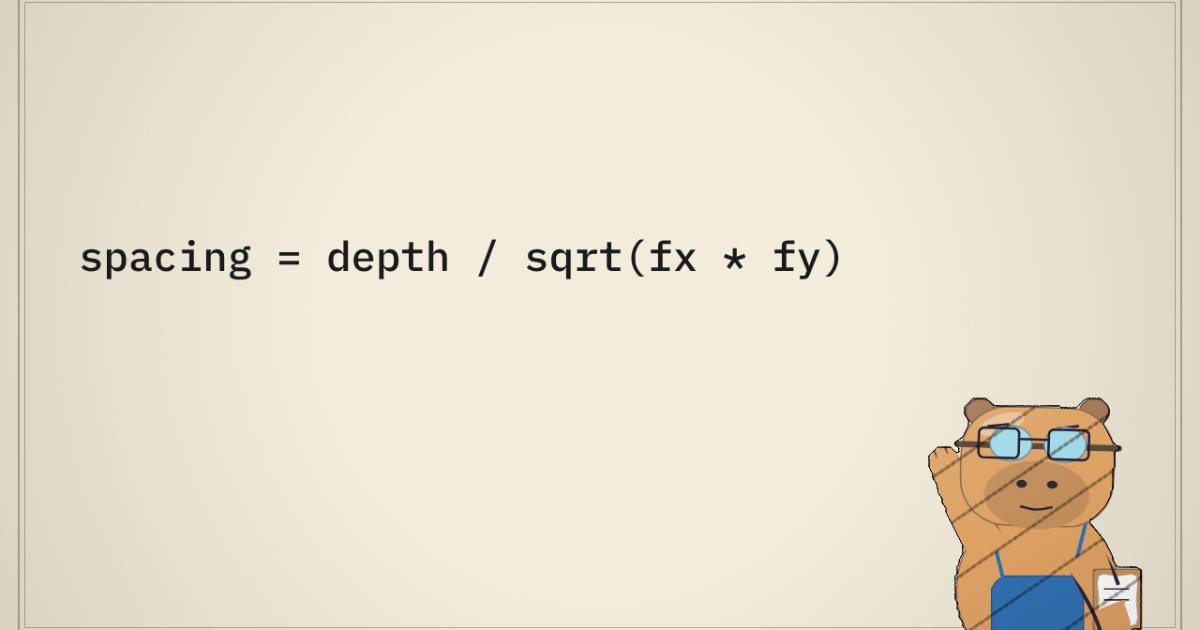
For two horizontally adjacent pixels at roughly the same depth $D$ , a pinhole camera with focal length $f_x$ (in pixels) puts their back-projected points $D / f_x$ apart. The paper takes the geometric mean of the two directions (Eq. 4):

d_i(\mathbf{u}) \approx \frac{D_i(\mathbf{u})}{\sqrt{f_{x,i}\, f_{y,i}}}

So spacing is depth divided by focal length in pixels. Metres matter, but so does the camera: a wider field of view or a lower image resolution means a smaller focal length in pixels, and the same wall at the same distance gets sparser Gaussians.

What everyone normalizes by instead

A geometry foundation model cannot know absolute scale from images, so it predicts the scene in some canonical frame. The common choice, which the paper calls RDNorm, divides everything by the mean distance of the reconstructed points from the reference camera (Eq. 5):

s_r = \frac{1}{N_p} \sum_{i,\,\mathbf{u}} \left\| \mathbf{P}_i(\mathbf{u}) \right\|_2

Feed-forward 3DGS methods built on these models (the paper lists DA3-GS, Mirror2-GS and others) inherit that frame and predict Gaussian scales inside it. After RDNorm the spacing is $D / (\sqrt{f_x f_y}\, s_r)$ (Eq. 7). The depth term is now relative, but the focal length is untouched, and the ratio between median depth and mean radial distance depends on the shape of the scene and where the cameras stand. Nothing pins the spacing.

Two panels. Left, labelled Radial Distance Normalization Space: a large-scale street scene and a small-scale bedroom both reach a box marked Consistent Radial Distance, but inside each 3D cube the gap between two neighbouring Gaussians differs, marked Inconsistent Gaussian Spacing, and after projection to 2D the predicted and target splat patterns disagree, marked Inconsistent Supervision Target. Right, labelled Gaussian Spacing Normalization Space, after a Scale Re-Normalization bar: the radial distances now differ but the Gaussian spacing in both cubes matches, and the projected targets agree. — The paper's framing of the problem: normalizing radial distance makes the scenes the same size but leaves the gap between neighbouring Gaussians different, so the same-looking image patch has different scale targets in different scenes. (paper, Figure 2).

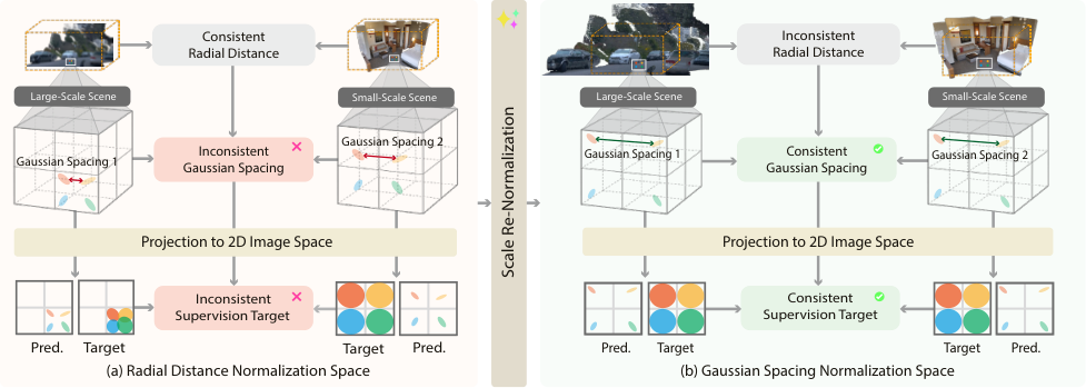
The consequence the paper draws is about supervision, not geometry. Two image patches that look the same (a stretch of plaster, a patch of grass) can need Gaussians of different size in normalized units, depending on which scene they came from. The rendering loss pushes the scale head toward one answer on one scene and a different answer on another. A head that hedges ends up too small on some scenes, which leaves holes, and too big on others, which blurs.

GSNorm is three lines

The fix is to choose the scene's scale factor so that the quantity the head has to predict against is the same everywhere. GSNorm sets the factor to the median spacing over every valid pixel of every view (Eq. 10):

s_g = \operatorname*{median}_{i,\,\mathbf{u}} \left( \frac{D_i(\mathbf{u})}{\sqrt{f_{x,i}\, f_{y,i}}} \right)

then divides depths and camera translations by it. Rotations and intrinsics stay. Because the median commutes with positive scaling, the median spacing after the division is exactly 1. The relative variation inside the scene (near ground versus far walls) is kept.

The release implements this in normalize_gaussian_spacing, in src/models/models/rasterization.py (measured, identical in the GitHub repository and the Space):

# src/models/models/rasterization.py (zju3dv/SplatAnything, c1a8992), abridged
focal = (intrinsics[..., 0, 0] * intrinsics[..., 1, 1]).clamp_min(0).sqrt()
spacing = depth[b] / focal[b, :, None, None]
factor[b] = self.spacing_target / spacing[valid].median()
depth = depth * factor[:, None, None, None]
poses[..., :3, 3] *= factor[:, None, None]

One detail differs from the paper. Eq. 9 pins the median spacing to 1; the code pins it to spacing_target=0.0013227513, which is 1/756 to the ten digits shown (measured), and 756 is the release's default input width. A constant factor changes nothing about the idea, but it changes how to read every other constant in the code. The Gaussian scale clamp in the paper's Eq. 17 is exp(s).clamp_max(0.3); with the median spacing at 1/756, 0.3 is about 227 median spacings (reasoned), a guard against blow-ups rather than a working bound. Read against Eq. 9 literally, it would have been under a third of a spacing.

Before the median, the function also reconciles the predicted depth with the camera translations, using the median ratio of pairwise camera-centre distances. In RGB-only mode the cameras are the geometry model's, so that ratio is 1 (reasoned from the code path), and only the spacing factor acts.

The inference path, shape by shape

The paper describes the model in two paragraphs and an equation. The release is short enough to read in full, and reading it answers several questions the paper leaves open. Here is one forward pass at the default 756 by 756 input, with shapes from the code (measured unless marked).

Preprocessing. Each image is cropped symmetrically around its principal point, rescaled, and cropped again to the target size, with the intrinsics updated at each step. Sizes must be multiples of 14, the patch size, so 756 gives a 54 by 54 grid of patches. Images go in as a tensor of shape $[B, S, 3, H, W]$ with values in 0 to 1.

Geometry. The frozen WorldMirror 2.0 returns, per view, a depth map $[B, S, H, W]$ , a 3 by 3 intrinsic matrix and a 4 by 4 camera-to-world pose, in its own radial-normalized frame. Its encoder also returns a list of token tensors that the Gaussian side reuses.

Alignment, then GSNorm. When you supply camera poses, the predicted depth has to be brought into the scale of your cameras first. The release does this with the median, over every pair of cameras $i, j$ , of

a = \operatorname*{median}_{i<j} \frac{\lVert \mathbf{C}^{\text{given}}_i - \mathbf{C}^{\text{given}}_j \rVert}{\lVert \mathbf{C}^{\text{pred}}_i - \mathbf{C}^{\text{pred}}_j \rVert}

where $\mathbf{C}$ are camera centres; depth is multiplied by $a$ . Pairs with a zero baseline in either frame are skipped, and if none are left (one view, or a cubemap whose faces share a centre) $a$ is 1. That guard is the code's answer to the CDNorm failure in Table 12: it never divides by a baseline that does not exist. The paper says the same alignment is used in training to render against ground-truth target cameras. Then comes GSNorm, as above: one factor $s$ per scene, depths and camera translations multiplied by it.

Features. The Gaussian backbone (a fine-tuned copy of the geometry transformer) yields four token layers of 2,048 channels on the 54 by 54 grid. GSFeatHead is a DPT-style decoder: four 1 by 1 projections to 256, 512, 1,024 and 1,024 channels, resized to 216, 108, 54 and 27 cells a side (a 4x and a 2x transposed convolution, an identity, a stride-2 convolution), fused coarse to fine by four refinement blocks at 256 channels, reduced to 128 channels and upsampled bilinearly to the full 756 by 756. A 7 by 7 convolution from the RGB image to 128 channels is added on top, so every pixel's feature carries its own colour at full resolution, not only what the 14-pixel patches saw.

Decoding. DPTDecoder turns that $[B \cdot S, 128, H, W]$ map into 12 channels with a 3 by 3 convolution to 256, a ReLU and a 1 by 1 convolution, eight views at a time to bound memory. The channels split 4, 3, 1, 3, 1:

rotation, a quaternion divided by its norm;
scale, $\min(e^{\hat{s}}, 0.3)$ per axis, in GSNorm units;
opacity, $\sigma(\hat{o})$ ;
colour, as a residual on the input pixel's own colour, stored as the degree-0 spherical-harmonic coefficient $(c - 0.5)/0.2821 + \Delta$ ;
merge weight, $\sigma(\hat{w})$ .

Centres are not predicted: each is the pixel back-projected with its normalized depth. At 756 by 756 that is 571,536 Gaussians per view (reasoned, $756^2$ ) before anything is filtered.

Filtering. With the shipped config, every scene loses the 0.5% of Gaussians whose largest scale axis is biggest (max_scale_pct: 99.5, applied as a rank cut, so it removes 0.5% of every scene whether or not anything is wrong with them). Sky masking is off unless you pass --sky_seg, which runs a separate 320 by 320 ONNX segmenter and drops sky pixels both from the GSNorm statistic and from the output; a view it calls more than 95% sky is left unmasked on the theory that the segmenter is wrong.

Merging and export. The survivors are averaged per voxel, as described below, and written as a PLY with Gaussians under opacity 0.05 removed.

One thing in that path disagrees with the paper. The paper says "the network predicts opacity" and that opacity "is activated using the sigmoid function" (reported). The release computes that sigmoid and then never uses it. In merge_voxels, the value written to the opacity field is the merge weight: for a voxel holding Gaussians with weights $w_k$ , opacity is $\sum_k w_k^2 / \sum_k w_k$ , and for a voxel with a single Gaussian that is just its own $w$ (measured, the line is values = weights if name == 'opacities' else scene[name]). The 0.05 export threshold is therefore a threshold on merge weights. A code comment calls this "the trained configuration's rule", so the checkpoint was presumably trained with it and the head has learned to put opacity into $w$ ; the fifth output channel group is dead weight at inference (reasoned). The rule has a consequence worth knowing if you edit the merge: it averages opacity instead of compositing it. Four Gaussians of opacity 0.5 in one voxel export as one Gaussian of opacity 0.5, where rendering the four unmerged would have accumulated about 0.94 along a ray through all of them (reasoned, $1 - 0.5^4$ ). Swap in a compositing rule and the model's surfaces will come out denser than it was trained for.

How it is trained

Three columns of 3D camera plots with strips of input and target frames under each. Interpolation Views: blue input cameras along a trajectory with red target cameras between them. Extrapolation Views (Off-Trajectory): red target cameras placed beyond the ends of the blue trajectory. Extrapolation Views (Zoom-In): red targets far from the blue cluster, looking closer at the scene. Top row is an outdoor street-art scene, bottom row a small bathroom. — The three target-view modes mixed during training: targets between the inputs, off the end of the trajectory, and zoomed in. The benchmark tests the second kind. (paper, Figure 9).

None of the training code is released, so this section is the paper's account (reported throughout, my arithmetic marked).

Schedule. 20,000 iterations on 64 NVIDIA H20 GPUs, a 500-step warm-up, learning rate $5 \times 10^{-6}$ for the Gaussian backbone and $2 \times 10^{-5}$ for the head, which is trained from scratch. The geometry model is frozen throughout.
Inputs. 4 to 32 source views per sample, with the input resolution varied from 504 to 1024. That resolution range is exactly why GSNorm's focal-length term matters during training, not only at test time: under RDNorm the same scene at the two ends of that range asks for scale targets about two times apart (reasoned, $1024/504 = 2.03$ ).
Loss. $\mathcal{L} = \lambda_{\text{MSE}}\,\mathcal{L}_{\text{MSE}} + \lambda_{\text{LPIPS}}\,\mathcal{L}_{\text{LPIPS}}$ with both weights 1, on target views rendered from ground-truth cameras after the baseline alignment above. There is no depth loss, which is consistent with the centres being fixed to the frozen geometry.
Data. 14 datasets, 22,659 scenes in all (reasoned, summed from Table 4), dominated by OmniWorld (10,464) and OmniObject3D (5,914), with MatrixCity contributing 8 city scenes and UnrealStereo4K 18.
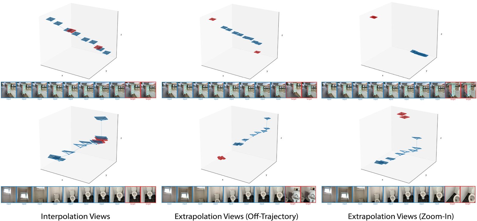
View sampling. Source views come from a mix of trajectory patterns (Figure 8 in the paper), and targets from the three modes in Figure 9. The ablation without this mix, sampling views at random and splitting them, costs 1.3% to 9.0% LPIPS depending on view count (reasoned, from Table 13).

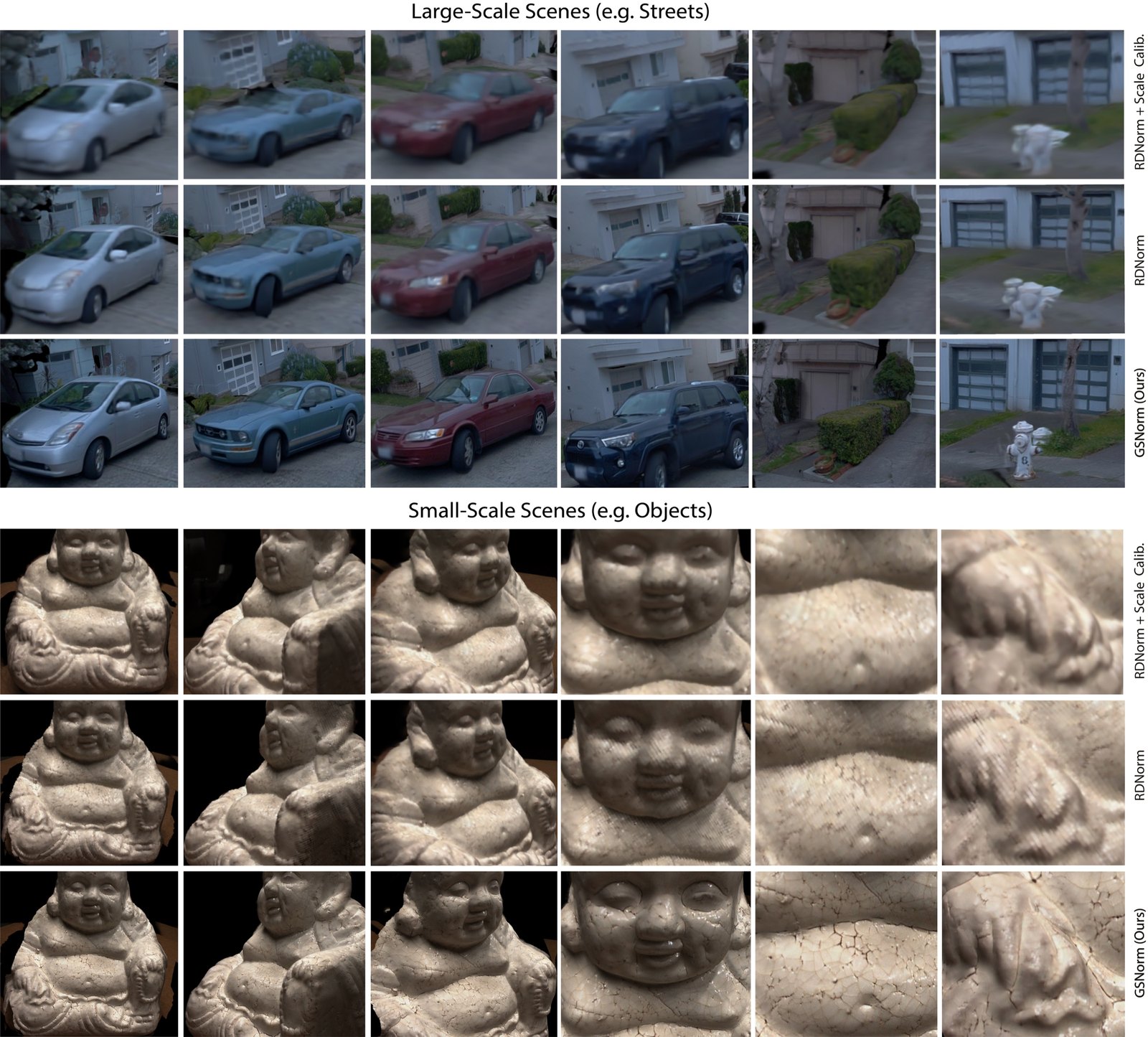
Table 13 makes a comparison possible that the paper does not draw. At four input views, training on Hypersim alone, 364 of the 22,659 scenes or 1.6%, costs 2.0% LPIPS (0.2499 against 0.2450); predicting centre offsets instead of fixing them costs 5.4%; freezing the Gaussian backbone costs 2.1% (reasoned, from the reported values). Swapping GSNorm for RDNorm, in Table 12, costs 11.9% (0.278 against 0.245). The paper calls fixed centres "the largest and most consistent gain" among its Table 13 choices, which is true of that table. Across both tables, the normalization is the largest effect the paper measures, about six times the effect of 62 times more training scenes. Those numbers come from two tables run separately, so read the ratio as an order of magnitude.

What the normalization does on six scenes

To see how much RDNorm actually leaves on the table, I wrote a ray caster in numpy (numpy 2.5.3, Python 3.13, CPU, under a second) for six captures with deliberately different geometry and cameras: an object on a ground plane filmed from an arc at 0.5 m, the same object at double the image width, an indoor room, a street canyon with an 80 m sky cut-off, an aerial pass at 120 m altitude, and a four-face cubemap from one point with a 95-degree field of view, the setting the paper's panorama appendix uses. Eight views each (four for the cubemap), 96 by 96 rays per view with the full-resolution focal length. For each, I computed the median spacing under RDNorm, under the two alternatives the paper's appendix tries (CDNorm: median camera-centre distance to the reference camera; DNorm: median depth), and under GSNorm.

median Gaussian spacing after normalizationnumpy toy · measured

RDNorm divides the scene by the mean distance to the reference camera. Largest over smallest median spacing across these scenes: 3.41x. Doubling the object's resolution from 504 to 1022 px halves its spacing under every norm except GSNorm. Synthetic scenes; the paper's own real-data plot is Figure 4.

The largest-to-smallest ratio of median spacing across the six scenes is 3.41x under RDNorm, 3.56x under DNorm and 9.41x under CDNorm (measured). GSNorm is 1x by construction. The paper's Figure 4, on real data grouped into object, indoor and outdoor scenes, reports 4.5x for RDNorm, from 0.30 to 1.36 relative to GSNorm (reported):

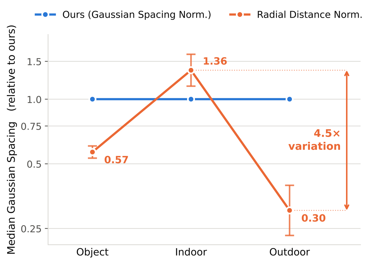
A line chart of median Gaussian spacing relative to GSNorm on a log axis, for three scene categories. The GSNorm line is flat at 1.0 for Object, Indoor and Outdoor. The Radial Distance Normalization line goes from 0.57 for Object up to 1.36 for Indoor and down to 0.30 for Outdoor, with error bars, and a bracket marks the gap as 4.5x variation. — Median Gaussian spacing per scene category on the paper's data. RDNorm's spread is 4.5x; my synthetic scenes give 3.41x, the same order. (paper, Figure 4).

Three things in the toy are worth naming because they are not visible in the paper's three-category plot.

Resolution alone moves it. The object at 1022 px has exactly half the RDNorm spacing of the same object at 504 px: 0.000678 against 0.001374 (measured). Nothing about the scene changed. The paper trains with input resolution varying from 504 to 1024, so under RDNorm the same training scene asks for two different scale targets depending on which resolution was drawn. GSNorm divides the focal length out.

Wide fields of view push it the other way. The cubemap faces have a focal length of 346 px at 756 px wide, against 540 px for the 70-degree room, and the cubemap has the largest RDNorm spacing of all six (measured). DNorm, which ignores focal length, has the same problem, which is the failure mode the paper's appendix shows for a roughly 100-degree scene.

CDNorm is undefined with one camera centre. The cubemap's four faces share a centre, so the median camera distance is zero. The same is true of a single input view. That is the likeliest reading of the paper's Table 12 row where CDNorm at one view scores DISTS 0.793 and LPIPS 1.027, three times worse than every other variant (reasoned).

What a confused scale head does

The second question is what those spreads cost. A real network sees image content and, through its backbone, some geometric context, so it is not blind to scale. The worst case is a head with no scale cue at all, which outputs one Gaussian size in normalized units for every pixel of every scene. I fitted that constant as the geometric mean of the ideal size over all six scenes (ideal sigma 0.7 times local spacing) and measured where each scene's pixels land against their own ideal.

one scale predictor, six scenesnumpy toy · worst case, no scale cue

capture 756 px

predicted / ideal scale0.52

sigma / Gaussian spacing0.37

alpha midway between centres0.49

toy pixels with holes / blur38% / 0%

Gaussians too small: gaps between centres

Dots are Gaussian centres one spacing apart; discs are their footprints out to three sigma. Ideal sigma is 0.7 spacings. The predictor never changes: only the space it is read in does. Try the cubemap or the object at 1022 px under RDNorm, then switch to GSNorm. The hole and blur shares count pixels whose local spacing puts them under half or over twice the ideal scale, so even GSNorm leaves the street's near ground and far walls mis-sized.

Under RDNorm, the cubemap's Gaussians come out at 0.52 of their ideal size, and 38% of its pixels fall under half the ideal, where the alpha between four neighbouring centres drops below 0.5 (measured). The object at 1022 px goes the other way, at 1.78 times its ideal (measured). Under GSNorm the same constant predictor lands at 0.98 of ideal at every scene's median (measured), and the cubemap's gap share goes to 0.

The toy also shows the limit. GSNorm aligns the median, not the distribution. The street canyon's spacing runs from 0.22 to 2.53 times its own median between the 10th and 90th percentiles (measured): near asphalt and far facades in one image. Under every normalization, the constant predictor leaves 15-24% of its pixels too small and 33-38% too large (measured). Removing the between-scene spread took the standard deviation of log(predicted / ideal) over all pixels from 0.585 to 0.488 (measured); the remainder is within-scene, and a scale head still has to learn it from content. GSNorm makes that problem the same problem everywhere. It does not solve it.

Sky inside the median

GSNorm's statistic is a median over "valid" pixels, and at inference the release decides validity with one test: depth above zero and a finite spacing (measured). A geometry model gives sky a large, finite depth, so unless you pass --sky_seg, every sky pixel is a valid sample. The training code is not released, so I cannot say what the statistic saw in training; the datasets in Table 4 come with depth maps in which sky is usually invalid, and the paper's Eq. 10 is written over valid pixels only (reasoned). The question is how far the default drifts from the masked version, and the toy answers it directly.

I built a street canyon (15 to 22 m walls, a 300 m street, sky above and beyond) filmed from 1.6 m, and an aerial pass at 120 m over a 5 km plain with 160 box buildings, then tilted the cameras up step by step. Eight views of 756 px at 60 degrees each, every fourth ray. For each tilt I computed the GSNorm factor twice, once with sky masked out of the median as --sky_seg does, once with it left in as the default does. The depth I give the sky does not matter as long as it is beyond the median, which is the point of a median.

sky inside the median: --sky_seg offnumpy toy · measured

pitch -15°

sky share: 30.3%
factor off by: 1.48x
non-sky median spacing: 0.68 × target
voxel, in those spacings: 2.01

The vertical axis is the GSNorm factor computed with sky masked out over the factor with sky left in, which is what the release does unless you pass --sky_seg. With sky masked, the non-sky median spacing is exactly the target and the voxel is 1.36 spacings wide. Past half the frame the median is itself a sky pixel and the factor is set by whatever depth the geometry model gives the sky, so the sweep stops before that. Synthetic scenes; not a run of the model.

The street, looking straight down the road, is 9.5% sky and the default factor is off by 1.08x; tilted up 25 degrees it is 27.7% sky and off by 1.29x (measured). The aerial pass is worse because its horizon carries more of the frame: at 30 degrees down it is 4.3% sky and off by 1.04x, at 15 degrees 30.3% and 1.48x, at 10 degrees 38.2% and 2.04x, at 5 degrees 45.7% and 3.51x (measured). Past half the frame the median is itself a sky value and the whole scene's scale is whatever the geometry model decided the sky's depth was. The curve is not smooth everywhere: the street at 10 degrees down is only 4.6% sky but off by 1.14x, because that tilt puts the median in a sparse stretch of the depth histogram between ground and walls, where a small shift in rank is a large shift in value (reasoned, from the toy's depth distribution).

What a 2x error does downstream is the problem GSNorm exists to remove. The real surfaces of the 10-degree aerial pass reach the Gaussian head at 0.49 of the spacing it is used to, and the voxel merge, set at 1.36 target spacings, now spans 2.78 of their spacings and averages away more detail (measured and reasoned from it). The fix is one flag, and the release's README offers it; the default leaves it off. For aerial and street captures with a visible horizon I would turn it on, for indoor scenes it makes no difference (reasoned).

The architecture around it

A left-to-right pipeline. Input aerial images of a city go into a Geometry Model marked frozen, which outputs depth maps and camera poses. A small point cloud in a dashed box is labelled Radial Distance Norm. Space, Mean(Radial Distance) = 1. A Scale-Renorm. block turns it into a larger point cloud labelled Gaussian Spacing Norm. Space, Median(Gaussian Spacing) = 1. A trainable Gaussian Model, which also receives the input images directly, produces the output 3DGS city scene. — SplatAnything's pipeline: a frozen WorldMirror 2.0 predicts depth and cameras, GSNorm rescales them, and a separately fine-tuned Gaussian model predicts per-pixel attributes. (paper, Figure 3).

The rest is close to InfiniSplat v2, with the geometry model swapped from Depth Anything 3 to Tencent's WorldMirror 2.0 (reported):

Frozen geometry. WorldMirror 2.0 predicts depth, intrinsics and camera poses. Its weights in the release are 1,263,337,852 parameters in FP32, 5.05 GB, in 1,593 tensors, about 0.92 billion of them in the visual geometry transformer (measured, safetensors header).
A second backbone for Gaussians. A copy of the geometry backbone is fine-tuned for appearance, and a small head trained from scratch decodes it. The release's decoder is two convolutions, 128 to 256 to 12 channels: 4 for rotation, 3 for log-scale, 1 opacity, 3 colour residual, 1 merge weight (measured, DPTDecoder).
Fixed centres. Every Gaussian sits on its back-projected pixel. The appendix's ablation finds letting the head predict offsets is the single most damaging change, LPIPS at one view going from 0.3667 to 0.4010 (reported, Table 13).
Colour is one RGB per Gaussian. The head predicts a residual on the input pixel colour and the export writes only the degree-0 spherical harmonic (measured, sh=((rgb - 0.5) / 0.2820… + residual_sh)), so view-dependent effects are baked in.
Voxel merge. Overlapping views put several Gaussians near the same point; the release averages them per voxel, weighted by the predicted merge weight. Opacity in the merged output is not the opacity channel: it is sum(w * w) / sum(w) over the merge weights, which a comment in the code calls the trained configuration's rule (measured).

The voxel merge is where GSNorm earns a second job. The voxel size is a constant in normalized units, and in GSNorm space a constant means a fixed multiple of the median spacing: the GitHub config's 0.002 is 1.51 median spacings, the Space's 0.0018 is 1.36 (reasoned, from 1/756). I ran my port of the merge at full resolution on the toy scenes. A single view keeps 53-78% of its Gaussians after merging at 0.0018; four overlapping views keep 24-38% (measured), so redundancy from extra views is what the merge removes. The object at 504 and 1022 px keeps the same 77.7% (measured): the merge is resolution-invariant in GSNorm space, where under RDNorm the same voxel would span twice as many pixel spacings at 1022 px as at 504 px (reasoned). The cubemap's four faces barely overlap, and four views keep 53.4% against 53.0% for one.

The two voxel sizes are a small loose end. The GitHub repository's configs/inference.yaml says 0.002 and its comment says the checkpoint was fine-tuned at that voxel; the Space's config says 0.0018 (measured). The Space is what the post links to.

What the merge keeps, by resolution and by view count

I ran the full merge port at full resolution on three of the new toy scenes (an object on a ground plane, a 6 by 8 m room filmed from a circle, a street canyon), sweeping input width from 504 to 1022 px at four views, and then view count from 1 to 16 at 756 px with the cameras spread over the same span, as the paper's benchmark does. For the resolution sweep I also counted what a voxel fixed in metres would keep, sized to match at 756 px: that is what a constant voxel in a radial-normalized space amounts to for one scene, and roughly what a merge in RDNorm space would do.

what the voxel merge keepsnumpy port of merge_voxels · measured

Grey: Gaussians before the merge, one per pixel. Green: after the merge at voxel 0.0018 in GSNorm space. From first to last row the merged count grows 4.11x while the raw count grows 4.11x. Because the voxel is a fixed number of pixel spacings, the merge keeps the same share at every resolution and the output grows with pixel count; a voxel fixed in metres (orange) would cap it. Synthetic ray-cast scenes, no model involved.

Three results (all measured):

The merge keeps a fixed share at any resolution. The room keeps 73.8% of its Gaussians at 504 px and 73.8% at 1022 px; the object 49.4% and 49.3%; the street 47.1% and 47.3%. The output therefore grows with pixel count: 4.11 times more Gaussians for the room at 1022 than at 504 px, the same 4.11 as the pixel ratio. A fixed-metre voxel caps that growth at 2.44 times for the room.
Extra views are mostly redundant, as intended. Going from 1 to 16 views in a fixed span multiplies the raw count by 16 and the merged count by 6.2 (object), 9.2 (street) and 11.2 (room). The room grows most because its views look in different directions and overlap least.
The factor depends on which views go in. The room keeps 54.5% with two views and 73.8% with four. The four-view set sees farther walls, which raises its median spacing, lowers the factor, and makes each fixed voxel hold fewer neighbours. Normalizing each of 16 room views on its own gives factors from 0.57 to 1.37 times the factor of all 16 together, a 2.4x spread; for the object and the street it is 1.02x. GSNorm normalizes the input set, not the scene, so the same room comes out at different scales depending on what was photographed.

The practical reading is about file size. Because GSNorm ties the voxel to pixel spacing, raising the input resolution does not buy you a coarser merge for free: at 1022 by 1022 and 32 views the release can emit tens of millions of Gaussians before the merge removes its share (reasoned, $32 \times 1022^2 = 33.4$ million raw). If you need a smaller PLY, the knob is gs_voxel_size in the config, at the price of running the checkpoint off the voxel it was fine-tuned at.

Checking the numbers

The cleanest evidence is the paper's own ablation: same architecture, same training, only the normalization space changed.

normalization ablation (Tables 3, 12)reported · lower is better

Same architecture and training, only the normalization space changes. GSNorm is lowest at every view count, by 3-13%. Rescaling RDNorm's predicted scales after the fact (scale calibration) is worse than not calibrating at all. CDNorm at one view is off the chart (DISTS 0.793, LPIPS 1.027): with a single camera there is no camera distance to normalize by.

GSNorm beats RDNorm at every input-view count in Table 12, by 3.1% to 13.4% depending on view count and metric (reasoned, from the reported values). The gap is smallest at the extremes: 4.5% DISTS at one view and 3.1% at 64 views, and largest in the 4-32 range the model was trained on. Two rows tell more than the winner:

Scale calibration makes RDNorm worse. Keeping RDNorm and rescaling the predicted Gaussian scales afterwards to match each scene's median spacing is the obvious cheap fix. It loses to plain RDNorm at every view count (LPIPS 0.309 against 0.278 at four views, reported). My constant-predictor toy cannot tell those two apart, because for a constant output a uniform rescale is exactly GSNorm. The paper's result says the benefit is in what the head learns when its targets are consistent, not in the output's units (reasoned).
DNorm is no better than RDNorm. Normalizing by median depth without the focal length gives 0.284 against 0.278 LPIPS at four views (reported), consistent with the toy's 3.56x spread being no smaller than RDNorm's.

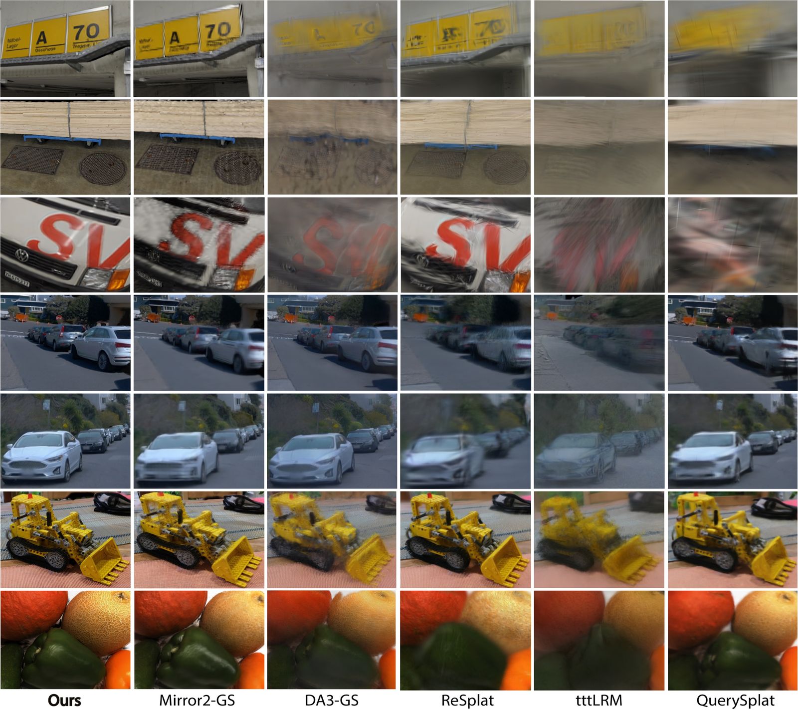
Against other methods, Table 1 averages each method over 4 to 64 input views on seven datasets with extrapolated target views. I parsed all fourteen tables in the arXiv HTML and recomputed Table 1 from the per-view-count Tables 5 to 9: all 182 cells (13 methods, 7 datasets, 2 metrics) match the mean of the per-view values to the third decimal (measured). One detail the caption leaves out: Table 9 has no ETH3D or DTU numbers at 64 views, so those two columns of Table 1 are averages over 4 to 32 views, not 4 to 64. In the RGB-only group, SplatAnything has the best number in 13 of 14 dataset-metric cells; with poses supplied, 12 of 14 (reasoned, counted from the table). The fairest comparison is Mirror2-GS, the same WorldMirror 2.0 with its own Gaussian head in its native radial-normalized space: SplatAnything's LPIPS is lower on all seven datasets, by 6.8% on ScanNet to 30.0% on ETH3D, 17.9% on average (reasoned). That gap mixes GSNorm with a fine-tuned backbone, 14 training datasets and a new view-sampling scheme, so only the ablation isolates the normalization.

Three caveats from the tables themselves:

PSNR tells a different story in places. ReSplat has the highest PSNR among posed methods at 4 to 32 views (19.03 to 19.67 against SplatAnything's 18.39 to 19.12, reported, Table 10). The paper's headline metrics are LPIPS and DISTS, following SHARP, on the argument that PSNR rewards blur. That is a fair argument and also the one every method that loses on PSNR makes.
The ETH3D LPIPS column is not a typo, but it does not measure what its neighbours do. Every method's ETH3D LPIPS in Table 1 is between 0.027 and 0.154 while its ETH3D DISTS is between 0.133 and 0.445 (reported). My first guess was a column slip in Table 1. It is not: the same low values appear in each per-view table (SplatAnything's ETH3D LPIPS is 0.047, 0.040, 0.037 and 0.071 at 4, 8, 16 and 32 views, reported), and Table 1 reproduces from them. What does stand out is agreement between the two metrics. Across the 13 methods, the Spearman rank correlation between DISTS and LPIPS is 0.62 to 0.98 on the other six datasets and 0.04 on ETH3D (measured, from Table 1). On ETH3D the two perceptual metrics rank the methods essentially independently. The ratio LPIPS over DISTS has a median of 0.69 to 1.59 elsewhere and 0.28 on ETH3D. Whatever the cause (image size, the high-resolution DSLR frames, a preprocessing step in the evaluation), the ETH3D LPIPS column carries little ranking signal, and the 30.0% gain above is the number I would trust least. On that column SplatAnything is third among pose-free methods, behind QuerySplat (0.031) and YoNoSplat (0.033); it is the one cell of fourteen it does not win.
Training on LPIPS does not explain the margin. The model is trained with an LPIPS loss and then scored on LPIPS, which could flatter it against methods trained otherwise. DISTS is not in its loss. Against Mirror2-GS, the average gain is 18.5% on DISTS and 17.9% on LPIPS (reasoned, from Table 1), so the held-out metric shows the same gap.
It is slower than its own base. On one H20 at 448 by 896, the median forward pass is 411 ms at 4 views and 11,037 ms at 64, against Mirror2-GS's 246 ms and 6,060 ms (reported, Table 11), about 1.7-1.8 times slower (reasoned). The second backbone is the likely cost. "Few seconds" holds up to about 32 views (3,991 ms).

A grid of novel-view renders, eight rows and six columns labelled Ours, Mirror2-GS, DA3-GS, ReSplat, tttLRM and QuerySplat. Rows show a yellow parking-garage sign reading A 70, a stack of timber over drain covers, the front of a white van with red lettering, two suburban streets with parked cars, a yellow toy bulldozer and a close-up of fruit. The first column is sharpest; the others show increasing blur, smearing and ghosting, with tttLRM and QuerySplat the most degraded. — The paper's qualitative comparison on extrapolated views with multi-view input. Mirror2-GS is the closest, as the tables say; the others smear text and fine texture. These are the authors' chosen examples. (paper, Figure 5).

A grid of rendered novel views in three column groups labelled RDNorm, RDNorm with scale calibration, and GSNorm, across rows of scenes: small objects, indoor rooms and large outdoor scenes. In object rows the RDNorm column shows holes and speckled gaps; the calibrated column fills them but looks soft; GSNorm is complete and sharp. In outdoor rows both RDNorm variants are blurry and GSNorm shows crisper building edges and foliage. — The ablation in pictures: RDNorm leaves holes on small object scenes and blurs large outdoor ones, calibration trades the holes for blur, GSNorm is sharper across scales. The paper's selection of examples. (paper, Figure 7).

What is released, and under what terms

zju3dv/SplatAnything@c1a8992 · snapshot 2026-11-10

tracked files

485

license: custom
branch: main
tests: 3 files
source: 231.9 kB
commit date: 2026-11-09

source by language

Python231.9 kB(47)

by size of tracked source at this commit, file counts in brackets; docs, data and vendored trees excluded

local clone, 2026-11-10 at c1a8992 — branch, commit, commitDate, fileCount, hasTests, languages, license, licenseFile, shallow, testFileCount

shallow clone: counts describe the pinned tree, not the history

Code: inference only. Every non-empty model file under src/models/ starts with # Modified for SplatAnything: inference-only release., and rasterization.py describes itself as decoding and voxel merging "(no rasterization or training)" (measured). There is no training loop, loss, rasterizer or data pipeline, so the paper's training and its benchmark cannot be reproduced from it. The view-sampling scheme and the benchmark split are described in the appendix, not shipped.
Weights. The model repository holds SplatAnything.ckpt (11.33 GB), worldmirror2.safetensors (5.05 GB) and an optional sky-segmentation ONNX model (176 MB) (measured). The checkpoint is a PyTorch Lightning zip with 5,107 entries, and its pickle names optimizer_states and lr_schedulers alongside state_dict (measured, read with pickletools, nothing executed). Part of those 11.33 GB is training state that inference never touches.
Licence, two answers. The Hugging Face model card says apache-2.0 (measured). The GitHub repository and the Space ship License.txt, the Tencent HunyuanWorld-Mirror Community License, which does not apply in the European Union, the United Kingdom or South Korea, requires a separate licence above one million monthly active users, and forbids using outputs to improve other models (measured). The geometry weights are WorldMirror 2.0, a Tencent model, so I would read the whole release under Tencent's terms until the authors reconcile the two (reasoned, not legal advice).
Hardware. The Space runs on a ZeroGPU A10G slot. The docs offer --device cpu "for slow smoke runs" (measured), which still means pulling 16.4 GB of weights. Inputs are multiples of 14 px; the default is 756 by 756.

ritianyu/SplatAnything@cea5713 · snapshot 2026-11-10

repo size

16.56 GB

license: apache-2.0
safetensors: 1 shard
largest file: 11.33 GB
files: 5
downloads: 0
likes: 2

repo last modified 2026-11-08

The repository's CPU tests (python -m unittest discover -s tests -v) need PyTorch, which this machine does not have, and installing it would have taken most of my disk budget, so I did not run them. My numpy port reproduces normalize_gaussian_spacing for RGB-only mode and the voxel-count part of merge_voxels; on every toy scene the median spacing after normalization comes out at 0.0013227513, the target, to the tenth digit (measured).

What I could not check

The list of things the second pass did not settle is as long as the list of things it did.

Nothing here ran the model. Every measurement above is either the paper's own number or my port of the release's inference code run on ray-cast depth. The ports are faithful line by line for the RGB-only path (the spacing statistic reproduces the target to ten digits, the merge uses the same flattened voxel key and the same weighted means), but a ray caster gives perfect depth, and WorldMirror 2.0 does not.
The training-time statistic. Whether training computed the GSNorm median over sky pixels or not decides whether the default inference setting matches training. The code that would answer it is not released.
What the sky depth is. My sky sweep only needs sky to be beyond the median. Past 50% sky the result depends on the depth the geometry model actually assigns, which needs the model.
The voxel key. The merge flattens 3D voxel indices into one 64-bit integer. I checked whether far points could overflow it: the product of the grid's three side lengths passes $2^{63}$ once points sit about 2,000 to 2,500 times the median depth from the scene, and the key then wraps. In 400,000 points with a shell out to 10,000 times the median depth, the wrapped keys produced zero collisions (measured), so the wrap behaves like a hash and is harmless in practice.
The ablation's variance. Tables 12 and 13 are single runs with no error bars. Gains of 2% (data scaling) are within what a second seed could move; the 12% of GSNorm over RDNorm at four views is much less likely to be.
The benchmark. The view selection and evaluation split are described, not shipped, so no number in Tables 1 to 13 can be rerun from the release.

Where it sits against prior work: InfiniSplat v2 on this site (InfiniSplat 2) is the direct predecessor and shares the per-pixel design; AnySplat, whose voxel merge this release inherits, normalizes in the geometry model's radial space, which is the RDNorm row of the ablation. The paper's contribution relative to both is the normalization and the training mix around it, not a new architecture.

Where it fits

If you build anything that predicts per-pixel Gaussians, or per-pixel anything with a physical size (surfels, splat radii, point sizes for a renderer), the transferable part is this paper's diagnosis, and it is cheap to check on your own data. Compute median(depth / sqrt(fx * fy)) per training scene in whatever frame your model works in. If that number varies by more than a factor of two or three across your data, and especially if it moves with image resolution, your scale head is being asked for different answers to the same question. Dividing by it costs one median.

What it does not fix is the spread inside a scene. A street, a corridor or anything with a ground plane running to the horizon has an order of magnitude of spacing within one image, and that is still the head's job. It is also no substitute for geometry: centres are fixed to the frozen model's depth, so whatever WorldMirror 2.0 gets wrong stays wrong. For the problem of drifting cameras, which is a different failure from mis-sized Gaussians, see VoxelTTO; for the rest of this autumn's feed-forward reconstruction papers, the 3D reconstruction roundup.

The novelty is small. It is one statistic replaced by a better-chosen one, the kind of fix that reads as obvious once someone has drawn Figure 2. That is also why it will last: the next feed-forward splatting model will have to pick a normalization, and now there is a measured reason to pick this one.