2026-11-12 · 34 min · 3d · gaussian-splatting · depth-estimation · datasets · benchmarks
A 5:00 narrated explainer, drawn in code. Every number and picture in it is this article's own; the sources are below.
› transcript
Why is there a point inside every Gaussian splat? And what happens if that point becomes a line? Hi, I'm Mirabel! Five 3D reconstruction papers from this week. We'll go deep on two of them. Chapter one. A point was a choice. A three D Gaussian is a point, blurred by a smooth kernel. That makes it something a renderer can differentiate. So a splat has two knobs: the kernel, and the thing being blurred. Swap the point for a segment, or a curve, and you get these soft tubes. A Gaussian is a point blurred by a kernel. Spaghetti Splatting blurs a line segment instead, and stays in closed form. Take a segment, two endpoints. Every point along it adds a Gaussian, and together they make a soft tube. Set the endpoints equal and it is an ordinary splat. Along a camera ray, that tube integrates to two error functions. No sampling. Each segment gets an opacity per pixel, composited like ordinary splats. Cut a segment in half, and the two halves composite to exactly the parent. The image does not move, so training can split freely. Here is the formula. Find the point on the segment closest to the ray. One error function counts the part of the segment before it. The other counts the part after. A ray passing beyond an end drives one negative, and the contribution fades. A triangle would need a much harder function here. A segment needs only erf, which is why the authors stop at curves. With points, a thin strand needs a Gaussian every two kernel widths, or it beads. A segment draws it with one primitive, and bends with a simulator. The article's toy draws one line with Gaussian points. Five points, and the density ripples by seventeen percent. Six points, two kernel widths apart: two point nine percent. Seven: zero point three. A thin strand needs a point every two widths. One segment, convolved with the same kernel: one primitive, and no ripple at all. Cut it in half, slide the halves apart and back. The halves sum to the parent exactly, so the image does not move, and training can split freely. On a real room, the point version draws the bicycle spokes as scattered dots. The segments run along the spokes and edges, like pencil strokes. On rooms it ties ordinary splatting, as a superset should. On hair it wins outright, by two point seven decibels, with no hair prior. Chapter two. One scale is not enough. Splats reconstruct geometry badly, so people add a depth network as a prior. Its depth is relative, so it is aligned with one global scale and shift. That leaves forty-one percent of pixels off. Give each of three regions its own scale and shift, and eighty-four point nine percent fit. With five, ninety-two point seven. The paper's scatter shows why. Predicted against true disparity falls on three different lines, one per surface. So AffineGS estimates a scale field that follows those surfaces. AffineGS models the relation per pixel. The network gives relative depth. The scale changes from surface to surface, not one number per image. A guided filter keeps both fields smooth within a surface. Without it they would copy the render. On a benchmark of indoor rooms, meshes score point seven one, against point two eight for a global fit the authors built themselves. Chapter three. Three more, briefly. Three more papers this week, briefly. Gaussian Grids hangs a feature grid on every 2D Gaussian. Another feeds a person's matching clicks into a point-map model. And one from Meta lets a stereo pair set metric depth, under a small decoder. Here is Click3R. A person clicks the same corner of a toaster in two photos. The base model alone splits the toaster in two. With one click, it is a single object. The article checked each claim against its own tables. Spaghetti's long connected strands average three and a half segments, and the code is not out yet. AffineGS initialises from sensor depth points, and tunes its filter scene by scene. And Gaussian Grids' point one bits per pixel is about point one three, by its own file sizes. Remember: the point inside a Gaussian was a choice. A segment keeps the closed form and draws thin things in one stroke. Segments instead of points, scale and shift per surface, and grids, clicks and stereo. Thanks for watching! Every source is in the full article. I'm Mirabel. Bye!
Why read this
Solidtop 85%Five splatting and 3D papers explained from the mechanism up, checked against their code, configs, checkpoints and data, with two live toys.
- Original analysis
- A new technique
- Explained from first principles
3D & spatialRuns on a consumer GPUMixed licencesResearch roundup
How this was scored
- Is it new?
- 2 of 3: A real new idea, method or capability
- Can I trust it?
- 2 of 3: Measures key facts from files, code or configs
- Can I run it?
- 1 of 3: API-only, gated or restrictive licence
- Will I understand it?
- 2 of 3: Mechanism from first principles with figures
- Can I act on it?
- 1 of 3: General advice
- Will it last?
- 1 of 3: Relevant for months
- Does it affect many?
- 1 of 3: A specialist community
- Only here?
- 2 of 3: A teardown or measurement few others did
Score 55 of 100, ranked 558 of 740 rated articles. Each question is answered 0–3 by hand, and a 3 is rare. How articles are scored
The last roundup asked how much of each release a reader could check from outside. This one starts somewhere else: what is the mechanism, in enough detail that you could implement it from the page. Four of the five papers are about Gaussian splatting. One changes what a primitive is (Spaghetti Splatting), one changes what supervises it (AffineGS), one moves the Gaussian into an image codec (Gaussian Grids), and one predicts splats from a stereo rig in a single pass (StereoSplat). The fifth, Click3R, is about the feed-forward point-map models that now sit in front of many splatting pipelines, and what to do when they get a scene wrong.
| Paper | What is new | Released on 12 November | What I checked |
|---|---|---|---|
| Spaghetti Splatting | The point inside a 3D Gaussian becomes a segment, then a polyline | Paper, project page and viewer; code dated 23 November | The closed form, subdivision, the margins in its table |
| AffineGS | Monocular depth aligned by a per-pixel scale and shift field | Code (Apache-2.0) with per-scene settings | The headline mesh number, the training scripts, the initialisation |
| Gaussian Grids | A feature grid attached to each 2D Gaussian, sized by local frequency | Paper; the code repository exists and is empty | The bits-per-pixel accounting, the ablation |
| Click3R | Cross-view clicks fed into DUSt3R through a small adapter | Code (MIT), weights, demo, benchmark lists and human clicks | The human clicks, the benchmark categories, the comparison with Pi3 |
| StereoSplat and XRStereo | Feed-forward splats on a frozen stereo model, and the synthetic data it trained on | Code and weights (CC BY-NC), the dataset (CC BY-NC) | The checkpoint header, the dataset card, three sequences read from a shard |
Spaghetti Splatting: a Gaussian whose point became a line
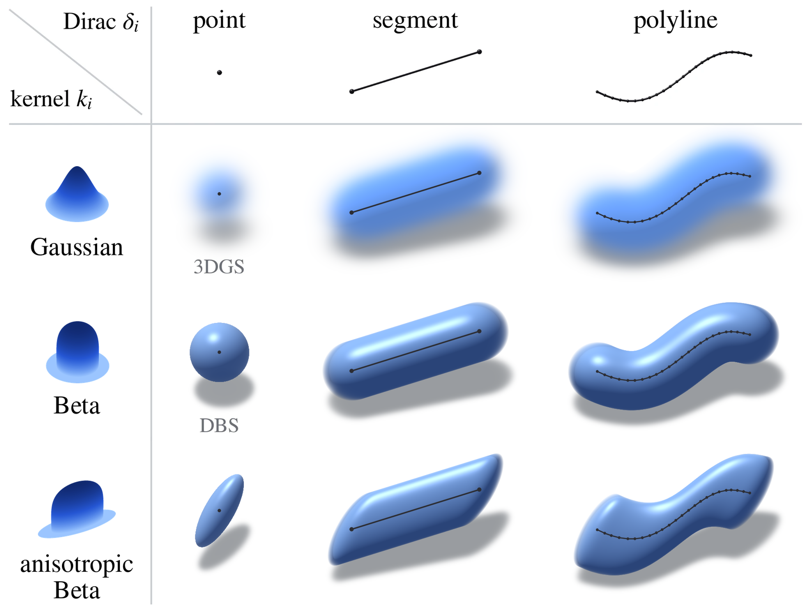
Rasterisers draw points, lines and triangles. A learned scene would be most useful as those primitives, but each of them is a Dirac mass: no extent, so a pixel beside it gets no gradient telling it to move closer. The paper, from Andrea Tagliasacchi's group at Simon Fraser with Wayve and Toronto, starts from an idea old enough to sit inside EWA splatting and Poisson reconstruction. Convolve the Dirac with a smooth kernel and you get a density that volume rendering can differentiate. A 3D Gaussian is exactly that, a Dirac at convolved with :
Written that way, 3DGS has two knobs. The kernel is one, and Deformable Beta Splatting already swapped the Gaussian for a compact Beta. The thing being convolved is the other. Points and triangles have been tried; this paper tries a segment.
From a segment to a density
A segment from to is the measure with : unit mass spread evenly along the line. Convolve it with the same Gaussian and scale by a density :
Every point of the segment contributes a Gaussian and the density is their sum. Set and the integral collapses to one Gaussian, so a 3DGS scene is a Spaghetti scene whose segments all have zero length. The "strict superset" claim is true by construction.
The ray integral is an error function
Volume rendering needs the optical depth along each ray . The density is already an integral over , so is a double integral, and because the Gaussian is non-negative the order can be swapped. A 3D Gaussian integrated along a line is a 1D Gaussian in , with a centre (the point of the segment closest to the ray, in the kernel's metric) and a precision that says how quickly the segment leaves the ray. A Gaussian integrated over is a difference of error functions:
is the kernel's line integral at the closest point. A ray far from the segment makes it tiny. A ray grazing the middle puts both error functions near one. A ray passing beyond an end drives one of them negative and the contribution fades. A triangle convolved with a Gaussian would need Owen's T function at this step; a segment needs only erf, which the authors give as the practical reason to stop at curves.
Evaluating that per primitive and per pixel is too slow for training, so the paper does what EWA splatting does for points. It linearises the camera projection once per frame at the segment's midpoint and scales the projected kernel along the segment by inverse depth, so the near end of a receding segment is drawn wider than the far end. Per-pixel work drops to a few screen-space quantities, and the Beta kernel fits too, since nothing now depends on the kernel being Gaussian in 3D. Mip-Splatting's anti-aliasing filters add to the projected covariance along the whole segment and come along for free.
Why a thin strand wants a segment
A strand of width drawn with points needs its points close together or it beads. The widget draws a line ten units long both ways in the image plane, using the paper's formula: one segment, or the same total mass as Gaussian points.
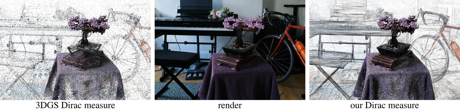
At the centre line of five points ripples by 17% of its mean, six points (spacing ) by 2.9%, seven by 0.3%. Those are my toy's numbers, and they say a line of length needs about Gaussians before it stops looking like a string of beads. A spoke one pixel wide wants a Gaussian every two pixels of its length. The segment needs one primitive and has no ripple. The paper's Figure 3 shows the same thing on a real scene: the 3DGS-MCMC centres on the bicycle spokes are scattered dots, and the Spaghetti segments run along the spokes.
Subdivision is exact, and this matters more for training than it looks. The convolution is linear, so cutting a segment at its midpoint into two halves that keep its density per unit length splits into two terms that sum to the original. Compositing the halves gives , the parent's transmittance, and the image does not move. The widget's last readout checks the density half of that: the two halves differ from the parent by about of its peak, which is rounding. Training keeps 3DGS-MCMC's relocation, splits long segments without a jump in the loss, clones short ones, and merges polylines whose endpoints come close, helped by a loss that pulls nearby endpoints together. The project page adds that each kernel's local x axis is its segment's direction, so when a simulator bends a strand, the kernels turn with it.
A tie on rooms, a clear win on hair
On Mip-NeRF 360 the paper's table has the Beta-kernel version at 28.78 dB PSNR, against 28.71 for DBS with the same Spherical Voronoi appearance model and 28.39 for 3DGS-MCMC. The Gaussian-kernel version leads on Shelly with 37.38 against 37.22 and on Fuzzy with 35.03 against 35.00. Those margins are 0.07, 0.16 and 0.03 dB: a tie on general scenes, which is what a superset of 3DGS ought to deliver. The concurrent Line Primitives method of Tojo et al. scores 8.66 dB on Mip-NeRF 360 because its lines keep a constant screen width and cannot represent a room.
Frame rate is close without being equal. On an RTX 4090 the paper measures 177 frames per second against 198 for 3DGS-MCMC on Mip-NeRF 360, 452 against 464 on Shelly and 415 against 422 on Fuzzy, between 89% and 98% of the point version.
Hair is where the primitive pays. On eight GeomHair hairstyles plus Cem Yuksel's curly model, rendered at 1200×800 with 88 training and 12 test views, it beats Gaussian Haircut by 2.7 dB (32.25 against 29.56) and by 14.3 points of strand F1 at 2 mm (61.2 against 46.9), with no hair prior, and the strands go straight into position-based dynamics.
One row of the ablation table deserves more attention than the paper gives it. The mean connected component is 3.50 segments for the full method and 1.00 with merging off, at PSNR 33.54 against 33.59. Merging costs nothing in image quality, but the "long connected strands" of the abstract average three and a half segments on these benchmarks. The conclusion is candid about it: "broader claims about automatically recovered topology require further evaluation".
Nothing runs yet. There is a project page with a web viewer of three scenes, the pasta among them, and a repository whose only file is a README reading "Code coming on November 23rd, 2026"; that was the state when I cloned it on 12 November.
13 November: a honeybee you can blow on. The project page's Viewer menu has a fourth entry, dated 12 November in the page source, after the two room models and the pasta: a honeybee, in a separate WebGPU viewer. @bettercallshaz posted a recording of it the next morning, crediting @taiyasaki, Dany Bittel and Will Eastcott. The page thanks Dany Bittel "for providing the bumblebee capture data, and Will Eastcott for showing a 3DGS reconstruction of it to the world" (the scene is named Honeybee). Eastcott's credit is for that earlier 3DGS version; this viewer is the authors' own WebGPU code, and none of its script modules mentions PlayCanvas.
The model is on Hugging Face as shaygeko/spaghetti-splatting-viewer. Its
header.json lists 500,000 segments, a run named
honeybee_xl_render_full_attr10_500k_turn35_30k_seed0_local_v1 and a
recorded_eval_psnr of 35.81 dB, on an evaluation split it does not describe.
The scene's files come to 119.4 MB, the wind simulation's data included. The
viewer has a Render, a Primitives and a Split view and a "Wind on the fur (live
simulation)" toggle. That is the paper's point that the strands go straight
into a simulator, made something you can watch move. It is also one scene the authors chose, with no
metric beyond that PSNR, and the stats line in the clip (12 fps at 768×388 on
an NVIDIA Turing card in a browser) says nothing about the paper's RTX 4090
numbers. Nothing else has moved: on 13 November the
repository still holds only
its README, last committed on 9 November, and the project page still shows
"ETA: Nov 23" under Code.
AffineGS: one scale and shift is not enough
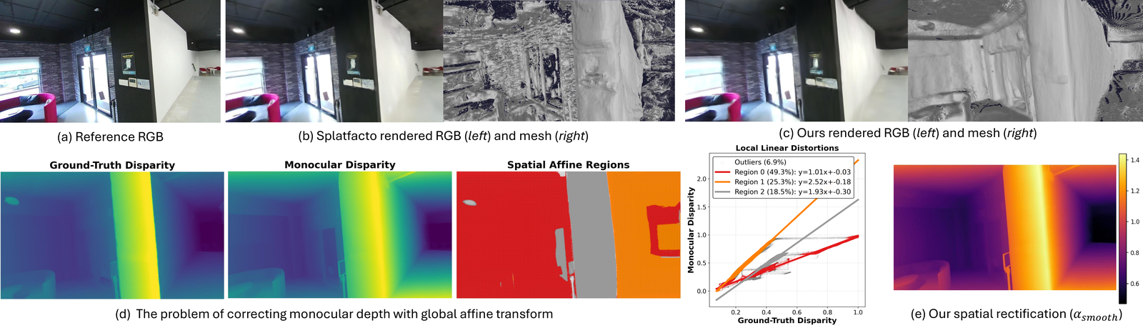
3DGS renders well and reconstructs geometry badly: layered, floating, overfit shells. The cheap fix is a monocular depth network as a prior. Depth Anything V2 and its peers predict relative depth, so the prior has to be aligned first, and the usual move (DRGS, and the monocular variant of DN-Splatter) is one global scale and shift solved by least squares. AffineGS, from dConstruct Robotics and NUS, accepted at NeurIPS 2026, measures how wrong that is. In its Table 1, on MuSHRoom, one affine transform leaves 41% of pixels outside a 0.02 residual. Split each image into three regions with their own transforms and 84.9% fit; with five, 92.7%. ScanNet++ behaves the same, 58.6% then 84.6% then 91.8%, with RMSE falling from 0.088 to 0.039.
Scale from a ratio of gradients
Let be the monocular disparity and the depth 3DGS currently renders. AffineGS models the relation per pixel:
Differentiate with respect to image position, assume the fields vary more slowly than depth (, ), and the shift drops out:
The local scale is a ratio of gradient magnitudes, clamped to its 5th and 95th percentiles, and the shift follows from the model. A guided filter then smooths both fields, with the disparity image as its guide and a radius of 550 to 650 pixels on MuSHRoom, so they stay flat inside a surface and break at the edges already has. The smoothed fields give a corrected depth , which is fitted once more with a global to the render so the scene cannot drift. It supervises through three losses. A gradient loss matches to in magnitude and direction. A second copy of it computes from the rendered normals and the intrinsics, which constrains the Gaussians' orientations and not only their depths. An L1 depth loss anchors the scale. Weights 0.1, 0.08 and 0.4, and every field is re-estimated each iteration.
Without the filter, the prior says nothing
Before smoothing, the fields are computed from the render, so they reproduce it. Substitute into the corrected depth and comes back unchanged; that is two lines of algebra on the paper's Eq. 1 and Eq. 9. A per-pixel affine field can fit anything. The prior carries information only because the guided filter forces the fields to be nearly constant across a surface, so the target takes its shape from within each surface and its scale from the render averaged over it. The filter radius is the real hyperparameter.
The widget is a one-row version of that argument, written for this article, not taken from the authors' code. Three surfaces, a monocular prediction that is exactly affine within each surface with different coefficients per surface, and a render that is right on average apart from a dent, a bump and blotchy noise.
With the surfaces disagreeing fully, one scale and shift fitted to the true depth leaves a mean error of 7.9 cm, with 46% of pixels within 5 cm. One fit per surface leaves none, since the toy's distortion is exactly piecewise affine; that is the paper's Table 1 in miniature. The estimator, which only sees the render, gives 4.6 cm against the render's own 5.5 cm at 5 cm of render noise, so the target pulls the render the right way. Give it a clean render and it lands at 3.8 cm against 3.3: nothing to add, as the algebra predicts. In one dimension a wide window hurts, 7.8 cm at a radius of 120 of 360 pixels, because the filter averages across surfaces. I could not reproduce the benefit of the paper's very large window in 1D, and I can't tell from here whether that is the toy's limit or a property of images, where a big 2D window still covers mostly one surface.
The 0.71 holds, with three asterisks
The X thread that circulated the paper quoted a MuSHRoom mesh F-score of 0.71 against 0.28 for DN-Splatter with monocular depth. Table 4 prints 0.7097 against 0.2765, so the quote is accurate. It is less than it sounds:
- The 0.28 is a baseline the authors built ("For a fair sensor-free comparison, we introduce DN-Splatter (Monodepth)"), meshed with the same TSDF fusion as AffineGS. Against published sensor-free methods the gap is smaller: 2DGS 0.6039, SuGaR 0.6378, Splatfacto 0.5835.
- "Sensor-free" describes the losses. The paper initialises the Gaussians
from "1M back-projected points from training dataset sensor depths",
following DN-Splatter, and the released data parser
(
dn_splatter/data/mushroom_dataparser.py) loads each scene'siphone_pointcloud.ply. - The settings are per scene. The released
run_train_paper.shsets the guided filter's radius to 550, 600 or 650 and its epsilon anywhere from 0.08 to 0.5 scene by scene, and halves all three loss weights onkokkoand quarters them onsauna, where its comment says the defaults "fill with floaters". The appendix lists the same values.
On ScanNet++, two scenes, AffineGS has the best normal consistency of the sensor-free methods (0.8308) and a lower F-score than 2DGS and SuGaR, 0.3207 against 0.4196 and 0.4367; the paper says so and blames a 5% depth shortfall on one scene. The sparse-view LLFF results, from a separate DRGS-based code base, are its strongest: mean PSNR 18.79 against DRGS's 17.31 at two views and 23.32 against 20.78 at five. Depth Abs Rel on MuSHRoom is 0.0551, against 0.3542 for the monocular DN-Splatter and 0.0228 for DN-Splatter with real sensor depth, so most of the gap to the sensor closes and some does not.
The code is out under Apache-2.0, built on DN-Splatter and Nerfstudio, last commit 6 November, with one script per table and a warning that the Depth Anything V2 Large weights it needs are CC BY-NC.
[NeurIPS 2026] AffineGS: Unlocking Accurate Geometry in 3DGS via Spatially Varying Affine Rectification
- license
- Apache-2.0
- branch
- main
- forks
- 4
- open issues
- 0
- source
- 824.9 kB
- commit date
- 2026-11-06
GitHub REST API, 2026-11-12 — branch, commit, commitDate, createdAt, description, forks, languages, license, openIssues, pushedAt, stars
Gaussian Grids: a feature grid on every Gaussian
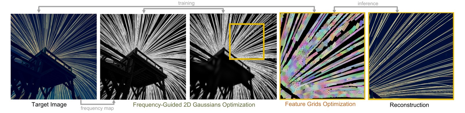
This one is about images, not scenes. Neural image codecs come in two families. Feature-grid methods (Instant-NGP, Neural Texture Compression) store a regular grid of learned features and decode with a small MLP: compact and fast, but they spend as much on sky as on a fence. Primitive methods (GaussianImage, Image-GS) put 2D Gaussians where the detail is, but each Gaussian carries its own position, shape and colour, and fine texture needs a great many of them. Gaussian-Grid, from NYU and Intel for WACV 2027, lets the Gaussians decide where capacity goes and stores the capacity as a small feature grid attached to each one. The summary that circulated had it as grids for flat regions and Gaussians for the rest. It is closer to the reverse: every Gaussian carries a grid, and one low-resolution "canvas" grid covers the smooth background.
Fit the frequency map first, the image second
For every pixel, take the 8×8 window around it, compute its 2D DFT and keep the largest magnitude that is not the DC term:
The map is high on texture and edges and near zero on flat colour. Stage one fits that map, not the image, with anisotropic 2D Gaussians that each carry a scalar frequency , under an L1 loss plus a pairwise overlap penalty that makes them tile the image instead of piling up: 3,000 steps in Taichi, starting from 800 to 2,300 Gaussians depending on the budget.
Stage two gives each Gaussian a share of the bit budget proportional to its frequency and its footprint,
raised where the local frequency vectors point many ways and lowered where they agree, with the grid's height and width following the Gaussian's anisotropy. The canvas takes 30% of the budget by default, more for flat images. A pixel samples the top Gaussian grids covering it, bilinearly and in each Gaussian's own frame, averages the valid samples, adds the canvas sample and decodes the 6-dimensional feature with a two-layer MLP of width 64. Grids train at 4 bits with quantisation-aware training, the MLP at 8, the Gaussians frozen to fp16, for 75,000 steps. The paper puts that at 24.3 minutes per image on an A100, which is the price of the format.
Better PSNR, worse LPIPS than a plain grid
On 100 DIV2K validation images it wins clearly at the lowest budget, 25.58 dB at 0.1 bits per pixel against 24.72 for the next method, and ties or edges ahead higher up: 29.36 against 29.36 at 0.4, 32.55 against 32.43 at 1.0. The ablation is less tidy. A single uniform grid given the whole budget reaches 32.08 dB at 1.0 bpp to the full method's 32.55, but the uniform grid wins on SSIM (0.9069 against 0.8999), MS-SSIM and LPIPS (0.0993 against 0.1167). The paper explains the trade plainly: capacity moves from flat regions to textured ones, PSNR goes up and the perceptual scores in smooth areas go down.
The bits-per-pixel accounting is where I would push back. The application section compares against JPEG plus ZIP on the same 100 images and lists dataset sizes. At "0.1 bpp" the 100 encoded images take 4.62 MB, 46.2 KB each, and the paper gives a decoded image as 8,306 KB, about 2.77 million RGB pixels. Divide one by the other and the nominal 0.1 is 0.13 bits per pixel; the other budgets come out near 0.43, 0.73 and 1.03. The excess is an almost constant 10 to 12 KB per image, which looks like the Gaussians and the decoder left out of the nominal budget, though the paper does not say. The JPEG comparison is size-matched, so it stands: 2.33 dB better than JPEG at the same size, decoded in 5.44 ms against 11.65 on an RTX 5080, and 47 KB over PCIe instead of 8,306 KB, the abstract's 176×. At 1.0 bpp JPEG is better by 1.00 dB. Whether the primitive baselines' 0.1 bpp counts the same bytes is the open question.
The paper says the source "is released at" a GitHub repository. The GitHub API shows that repository was created on 21 October with a size of zero, and cloning it returns an empty repository.
Click3R: a few clicks into DUSt3R
DUSt3R and its successors predict a point map for two images in one forward pass. When they get it wrong (repeated texture, a symmetric building, a large viewpoint change) the only options are to accept the output or fall back to optimisation. Click3R, from the University of Virginia, adds an input: a few correspondences a person clicks, one point in each image per click, the way SAM takes clicks for segmentation.
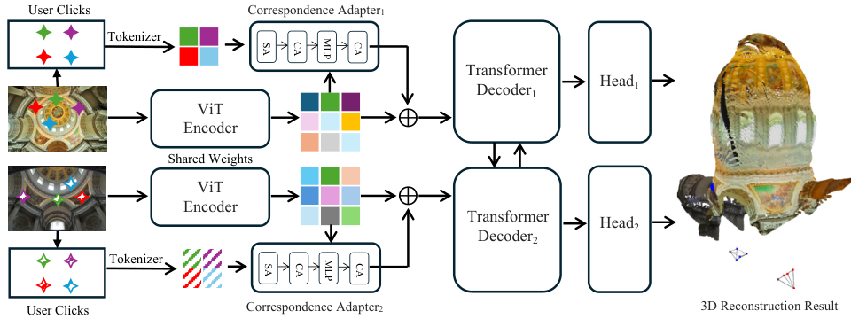
How a click becomes a token
DUSt3R encodes each image with a shared ViT-Large (24 blocks, width 1024), projects the patch tokens to width 768 and runs two 12-block decoders that cross-attend to each other. Click3R sits between the projection and the first decoder block. Each clicked point becomes a token made of three parts: its coordinates, normalised to the token grid and encoded with SAM's random Fourier features; a learned embedding for which view it is in; and a learned embedding for which click it is, shared by both ends. The pair embedding is what tells the network that this point in image one is that point in image two. Per view, a two-layer adapter runs self-attention over the clicks, cross-attention from clicks to image tokens, an MLP, and cross-attention from image tokens back to clicks, and its output updates the image tokens. The image positional encoding uses the same Fourier features, so a click and the patch under it share one coordinate space. With no clicks the adapter is the identity.
The adapter is small; the training is not. Everything is trained end to end from CroCo v2 with simulated clicks, a random number per sample, and freezing DUSt3R to train only the adapter is the worst of the three variants the paper tried, 71.2 mAA@30 against 75.1. The README lists the checkpoint at 566.6M parameters against 532.3M for DUSt3R retrained on the same data, so the clicks cost about 34M parameters. Inputs are 224×224.
Hard3DBench is mostly wide baselines
The authors built Hard3DBench to make DUSt3R fail: 404 in-distribution and
300 out-of-distribution pairs, plus 5-view tuples. The category file they
released shows what "hard" mostly means. In categories.json, 371 of the 404
in-distribution pairs and 235 of the 300 out-of-distribution pairs are
tagged large baseline, many of them large viewpoint as well. Symmetric and
textureless scenes, named in the abstract, are not categories at all. On the
out-of-distribution pairs the retrained DUSt3R scores 52.6 mAA@30; one click
gives 56.6, four give 60.4, eight give 62.4.
Pi3 at the same 224 resolution, with no clicks, scores 71.1 on those pairs, and VGGT at its native 518 scores 81.3. The paper lists them as references rather than baselines because they are larger and trained on more data, which is fair. The practical reading is still that clicks fix DUSt3R, not that they beat a stronger model. The standard-benchmark gains that look largest also come from oracle click selection. "1p_best5" picks the best of five random clicks by reconstruction loss; the "grid oracle" tries one click in each of about 256 cells and keeps whichever most reduces the pose error. That is where 84.27 to 92.75 on ARKitScenes comes from. It measures headroom, not what a person achieves.
What one person's clicks did, and on what
The human study is the part that measures a person. One annotator, 100 out-of-distribution pairs, no access to depth or poses: median rotation error falls from 17.30° to 8.78°, mAA@30 rises from 36.2 to 56.2, and four random ground-truth clicks reach 8.40°. The paper's "96% of the gap" is , so that checks.
I read the released human_clicks.json. It holds 377 click pairs over the
100 image pairs, a mean of 3.77 and a range of 1 to 7, which matches the
paper's 3.8. It also shows that 77 of the 100 pairs come from DTU, 12 from
ETH3D, 4 each from NRGBD and 7-Scenes and 3 from ScanNet. DTU is tabletop
objects shot from a robot arm, so the human result is mostly a result about
objects. The perturbation analysis adds a practical limit: predictions start
following a wrong click once it is off by half of a 16-pixel patch, 8 pixels.
Of the five, this is the release with the least missing: training and evaluation code (MIT), weights (CC BY-NC-SA 4.0), a Gradio demo on Hugging Face Spaces, and Hard3DBench's sample lists, labels, clicks and unrounded paper numbers (CC BY 4.0). The benchmark does not redistribute images; the code prepares them from the source datasets.
[NeurIPS 2026] Click3R: Interactive Stereo 3D Reconstruction with Sparse Correspondence Clicks
- license
- MIT
- branch
- main
- forks
- 0
- open issues
- 0
- source
- 576.8 kB
- commit date
- 2026-11-10
GitHub REST API, 2026-11-12 — branch, commit, commitDate, createdAt, description, forks, homepage, languages, license, openIssues, pushedAt, stars, topics
StereoSplat and XRStereo: let the rig set the scale
Feed-forward splatting models (pixelSplat, MVSplat, DepthSplat, AnySplat) take a few images and emit Gaussians in one pass. Their geometry is up to scale, or comes from cost volumes that blur with distance. A headset or a robot usually has something better: a calibrated stereo pair, from which metric depth is for focal length , baseline and disparity . StereoSplat, from Meta and the University of Amsterdam, builds the splatting model around that.

Four stages on top of a frozen stereo model
- Grounding. A frozen FoundationStereo computes the left view's disparity. For the right view, flip both images and swap them so the right image plays "left", then flip the output back. Depth for both views is , and the same pass yields a four-level feature pyramid.
- Cross-view fusion. At every pyramid level and pixel position, the features of all views form a sequence of length for a small transformer. Attention is per pixel whatever the image size, and zero-initialised output projections make it start as the identity.
- A gated depth. The decoder upsamples to full resolution, predicts Gaussian attributes per pixel and a refined depth , and blends it with the stereo depth by one learned scalar, , initialised to trust the stereo.
- Merging in inverse depth. The Gaussians overlap heavily across frames. Each centre maps to and is hashed on a grid of size , so a cell is about wide and deep: fine nearby, coarse far away. Quantised colour, scale and opacity join the hash key so a cell never merges across an edge, and Gaussians in a cell are averaged with predicted softmax weights that start uniform.
Training renders the merged Gaussians into held-out views with gsplat and supervises colour (L1, SSIM, LPIPS) and metric depth (L1), on synthetic data only: XRStereo, TartanAir and Infinigen.
The trained part is 5.1 million parameters
I read the header of stereosplat_v1.safetensors on Hugging Face with two
range requests. It holds 317 tensors and 5,143,087 parameters, all float32,
about a third of them in the three cross-view fusion blocks. The config
stored in the header sets spherical-harmonic degree 0, so colour is not view
dependent, and a maximum depth of 80. What StereoSplat trains is a small head;
the geometry comes from FoundationStereo, which the README has you clone
separately under NVIDIA's own licence.
On KITTI, outside its training data, the paper reports novel-view depth Abs Rel of 0.04 against DepthSplat's 0.13, δ1 of 96.0 against 79.8, and PSNR of 25.2 against 22.3 for pixelSplat. On Infinigen, Abs Rel is 0.03 against 0.21. Read the protocol before reading those as a contest. The baselines run their public checkpoints, not retrained on stereo; MVSplat, pixelSplat and VicaSplat run at their native 256×256 against StereoSplat's 320×640; and the pose-free ones work in a normalised space where metric depth means nothing. The pose-aware baselines do get ground-truth poses while StereoSplat uses MAC-VO odometry. The geometry gap is mostly the rig's information, which is the paper's thesis, and it says little about whether the decoder is better at what the baselines attempt. The aggregation's compression rate in the ablation is a modest 1.6.
XRStereo: what the paper says and what was uploaded
The paper describes 137k frames in 20k sequences across 9 indoor and 4
outdoor environments, objects drawn from 200 assets, rendered at 1K with
horizontal fields of view from 50 to 130 degrees and baselines from 40 to
120 mm. The Hugging Face card and its manifest.json describe the upload:
17,922 sequences of 5 stereo frames, 89,610 stereo frames and 179,220 images
at 1024×1024, 372.8 GB in 72 tar shards, CC BY-NC 4.0, and "This release is
the StereoSplat training split". Nothing published reconciles the paper's
137k frames with the upload's 89,610.
I pulled the first 40 MB of shard 0 with a range request, which holds three sequences. Their focal lengths give horizontal fields of view of exactly 70, 60 and 80 degrees, their baselines are 120, 60 and 40 mm, and the camera moves 4.7, 11 and 8 cm between frames. Left and right disparities agree within one pixel on 91% to 100% of pixels, the rest being occlusion. The first sequence is a blank wall about 0.6 m away. The scenes are rooms full of floating, randomly posed objects, closer to FlyingThings than to a home.
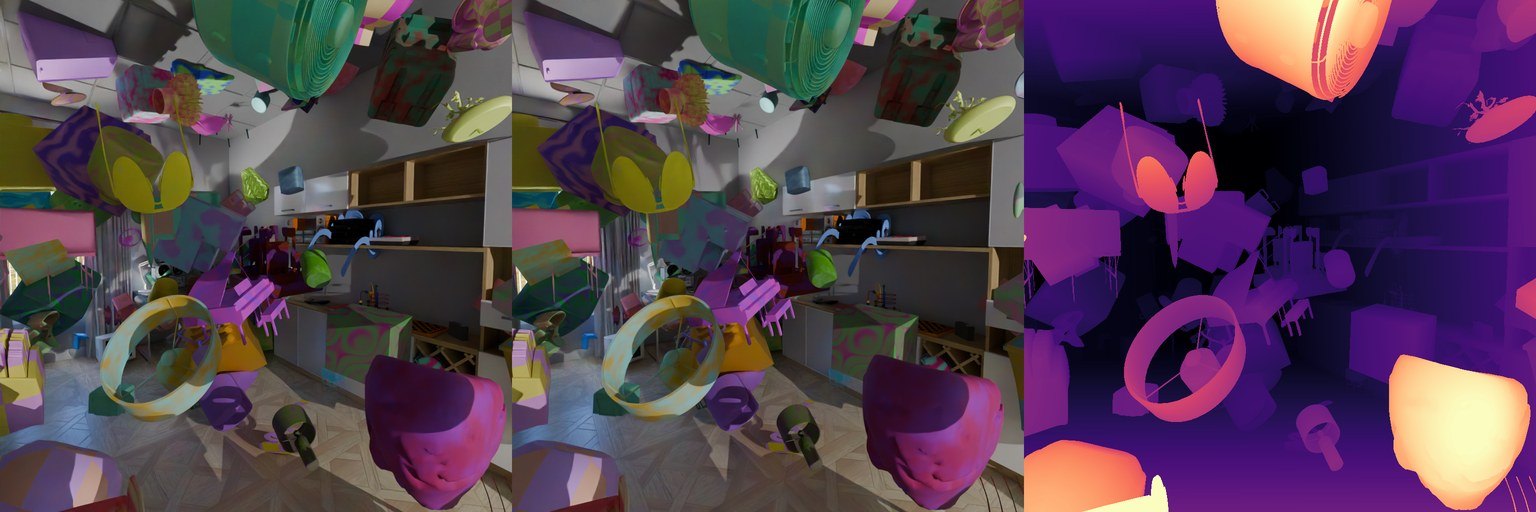
Everything here is non-commercial. The code (facebookresearch/stereo-splat,
89 files, last commit 11 November), the weights and the dataset are all CC BY-NC
4.0, while the project page still says code is coming soon.
Source code for the NeurIPS 2026 paper StereoSplat Metric-Scale Novel View Synthesis via Stereo-Grounded Gaussian Splatting
- license
- custom
- branch
- main
- forks
- 0
- open issues
- 0
- source
- 395.4 kB
- commit date
- 2026-11-11
GitHub REST API, 2026-11-12 — branch, commit, commitDate, createdAt, description, forks, languages, license, openIssues, pushedAt, stars
Where I'd spend time
If you build splatting pipelines, read Spaghetti Splatting and AffineGS properly; skim the rest.
Spaghetti Splatting is the idea I expect to outlast its paper. The point inside a Gaussian was a choice, and a segment keeps everything that made the point convenient: a closed form, the EWA linearisation, anti-aliasing, and a subdivision that does not change the image. On rooms it ties 3DGS, as a superset should. On hair, spokes and wires it wins outright. The connected strands are shorter than the abstract implies, and there is no code until 23 November, so hold judgement on the simulation story until you can run it.
AffineGS makes a point I agree with: a single global scale and shift throws away most of what a monocular prior knows. The method holds up, with three asterisks on its headline number: a baseline the authors built, a sensor point cloud at initialisation, and a filter tuned scene by scene. If you already regularise splats with Depth Anything, the per-surface alignment is the part to steal; the code is Apache-2.0.
Gaussian Grids is a careful hybrid, but I don't buy the 0.1 bpp headline until the Gaussians and the decoder are counted, and there is no code to check it against. Click3R is the most complete release of the week and the easiest to try in the browser. Its own data says the human study is mostly DTU objects and that Pi3 without clicks still leads on its hard pairs, so I would put clicks on Pi3 before I put them on DUSt3R. StereoSplat's geometry numbers come from information the baselines never had. What I would actually download is XRStereo, if non-commercial use is enough for you.
For where these primitives end up, see SplatAnything, InfiniSplat v2, the capture side in Gaussian-splat capture in practice, and how splat colour is stored in Gaussian-splat colour.