2026-11-12 · 22 min · retrieval · multimodal · decision-models · vision-language-models · video-understanding · benchmarks
A 5:13 narrated explainer, drawn in code. Every number and picture in it is this article's own; the sources are below.
› transcript
One model searches a corpus of millions, and answers yes or no questions. How can one cosine do both? Hi, I'm Fenna! Meta's MetaEncoder turns a thirty billion parameter chat model into an embedding model. Let's see how, and what it can decide. Chapter one. Three ways to score a candidate. A cross-encoder reads the request with each candidate. A constrained decoder lists every option as a letter. Both are accurate, and neither can cache a thing. A bi-encoder embeds the request and each candidate separately and compares them by cosine. Candidates are embedded once, so it scales to millions. MetaEncoder is one of these. Chapter two. One tower, not two. Pictures go through Muse Glimmer's own vision tower. Every twenty-eight by twenty-eight pixels become one token at the decoder's width. Those tokens sit in one sequence with the text: the task instruction, then the input. The same fifty-two layer decoder reads it all. Nothing is averaged. Under causal attention, only the last token has seen everything, so its hidden state is the embedding. Version one adds a square head and normalises to unit length. Queries, documents and answer options all come out the same way. Hand the wrapper a video as a list of frames. It keeps eight, evenly spaced, first and last included. Each one goes in as its own image. There is no temporal pooling at all. The decoder reads the frames and the question in order. Training never went past sixteen thousand tokens, and inputs are never truncated. Out come six thousand six hundred and fifty-six numbers: about twenty-six kilobytes in float thirty-two, for every vector you store. This is what the model sees: eight frames of a test clip. Asked where the dog is sitting, it puts almost all its probability on couch. Chapter three. A decision is a retrieval. Here is a choice question from the model card. The request and each option are embedded separately, by the same network, as unit vectors. The option pointing most nearly the same way as the request has the largest cosine. That is the answer. To turn cosines into probabilities, divide by the training temperature, point zero two, and take a softmax. A small cosine gap becomes a confident answer. Raise the temperature and the bars flatten, but the winner never moves. Calibration changes how sure the model sounds, never what it answers. Here is the formula. Training uses the same softmax. Each request is scored against its candidates. Unlike CLIP, it runs in one direction only. A candidate like No never has to find its question. For search, the negatives are everyone else's documents in the batch. For a decision, they are the row's own wrong options. The loss is the evaluation. Chapter four. Putting the options in the question. A bi-encoder's request never sees the options. So list them in the prompt. On MMLU that lifts accuracy from point five six to point seven five, and letter plus text adds three points. Chapter five. What the numbers say. This table on the card is all the evidence for version one. On decisions and multiple choice, it leads most rows. Retrieval is closer than the post says. A clear win on text search, a whisker on images, a tie on video, and a loss on documents, against a model a third its size. And on the hardest decision split, version one went backwards. Eighty-two right became seventy-six, while Open-Jev gets eighty-five. Chapter six. Where one vector runs out. The paper tests itself against its own base model. Allowed to think before answering, the decoder jumps from about point five to point seven two on MMMU. Give MetaEncoder that reasoning as context and it climbs from point five seven to point seven one. One forward pass cannot do the thinking itself. Three things to know before you use it. The paper describes the earlier checkpoint. Version one's evidence is a single picture. The evaluation repository's own reference file puts video retrieval four points below the paper. And version one ships with no licence at all. Version zero is Apache two point oh. A decision can be a retrieval over a short list. Embed the options once, write them into the question, and pick by cosine. One chat model, read at its last token. Decisions as a softmax over cosines. A fast first pass, reasoning elsewhere. Thanks for watching! Every source is in the full article. I'm Fenna. Bye!
Why read this
Notabletop 60%Reads MetaEncoder from its headers and code (one tower, last-token pooling, video as 8 images, softmax over cos/0.02) and checks what the v1 table hides.
- Original analysis
- Widely used
- A lasting reference
Vision & multimodalNeeds datacenter GPUsNo licencePractitioner model
How this was scored
- Is it new?
- 2 of 3: A real new idea, method or capability
- Can I trust it?
- 2 of 3: Measures key facts from files, code or configs
- Can I run it?
- 1 of 3: API-only, gated or restrictive licence
- Will I understand it?
- 2 of 3: Mechanism from first principles with figures
- Can I act on it?
- 2 of 3: A concrete recipe, numbers or comparison
- Will it last?
- 2 of 3: A reference for a year or more
- Does it affect many?
- 2 of 3: A widely used model, tool or lab release
- Only here?
- 2 of 3: A teardown or measurement few others did
Score 66 of 100, ranked 253 of 740 rated articles. Each question is answered 0–3 by hand, and a 3 is rare. How articles are scored
On 12 November DailyPapers posted that Meta had released MetaEncoder, "a unified multimodal encoder for text, images and video, with SOTA retrieval and decision support". The post carries one image, a benchmark table, and no video; the account's own reply links facebook/meta-encoder-v1.
"Encoder" suggests something like CLIP: a small image tower, a small text tower, a shared space. MetaEncoder is nothing like that. It is Meta's Muse Glimmer 30B, a chat model, with its output layer removed and the hidden state of its last token read out as the embedding. The same model encodes queries, documents, pictures, video frames and the answer options of a classification question. "Decision support" means exactly that: a yes/no or multiple-choice question is answered by retrieving the closest option.
The parts are all public. What follows is how it works, read from the code and the weights, and then what the numbers behind "SOTA" actually are.
| Weights | facebook/meta-encoder-v1, published 12 November, 11 bf16 shards plus embedding_head.safetensors. No licence file and no licence field |
| Predecessor | facebook/meta-encoder (v0), 30 September, Apache-2.0 plus Muse Glimmer's usage policy, gated |
| Paper | arXiv 2610.11316, MetaEncoder: Exploring the Limit of Bi-Encoders for Multimodal System One Decision Making with Natural Language Interface, Jianpeng Cheng and 13 co-authors, Meta AI, 8 October. It describes v0 |
| Evaluation code | facebook/meta-encoder-eval, Apache-2.0, read at commit ecc7792 (9 October), written for v0 |
| Demo | facebook/meta-encoder-space, a precomputed gallery from v0 |
| Base | meta-models/Muse-Glimmer-30B, Apache-2.0 |
| Size | 28,476,097,536 parameters in v1, by my count of the safetensors headers; one 80 GB GPU in bf16, per the card |
- architecture
- MuseGlimmerModel
- task
- feature-extraction
- library
- transformers
- safetensors
- 12 shards
- largest file
- 5.28 GB
- files
- 23
- downloads
- 5
- likes
- 14
repo last modified 2026-11-12
Three ways to score a candidate
Strip away the modalities and every task MetaEncoder is evaluated on has the same shape. There is a request (a search query, a question about an image, a support ticket and an instruction) and a set of candidates (a corpus of passages, four answer options, the labels "spam" and "legitimate"). The model has to rank the candidates. The paper's related-work section lays out the three ways a language-model backbone can do that, and the choice between them is the whole design.
A cross-encoder reads the request and one candidate together and emits a relevance score. Full attention between the two makes it the most accurate of the three, which is why it is the standard reranker. It is also the most expensive: candidates cost forward passes over the shared request, and nothing about a candidate can be computed ahead of time.
A constrained decoder puts the request and every candidate, lettered A to Z, into one prompt and reads the next-token probabilities of the letters. That is how MMLU has always been scored, and it is what Jev-style System One models do with a trained head instead of letters. One pass covers every option, and options can be compared with each other. But the option set is bounded by the alphabet and the context window, accuracy moves with option order, and the output is a distribution over positions, not anything you can store.
A bi-encoder embeds the request and each candidate separately, and scores them by cosine similarity. Because a candidate's embedding never depends on the request, it can be computed once and indexed. Scoring candidates costs one forward pass for the request plus dot products, and can be millions. The price is that everything the request knows has to fit through one vector, and the request never sees what it is being compared against.

Every embedding model is a bi-encoder, and so is every classifier that compares an input with label embeddings. CLIP did zero-shot ImageNet that way in 2021. The paper's question is how far the bi-encoder can be pushed as a general decision maker, with a 30B backbone and some prompt engineering to claw back what the cross-encoder gets for free.
The loss, in one direction
Training a bi-encoder is contrastive. Take a batch of requests , each with its correct candidate . Embed everything, normalise to unit length, and score with . The paper's Equation 2 is an InfoNCE loss:
It is a softmax classifier whose classes are the candidates in front of it. The temperature sets how sharp it is. Cosines live in , so without a temperature the logits could differ by at most 2 and the softmax could never be confident. Dividing by multiplies them by 50: a cosine gap of 0.05 becomes 2.5 in logits, odds of about 12 to 1. The paper never states its temperature. The number comes from v1: the card says decision probabilities are softmax(score / 0.02), "the contrastive training temperature", and the wrapper sets TRAINED_TEMPERATURE = 0.02.
Two details separate this from the losses most readers know.
It runs in one direction only. CLIP's loss is symmetric: each image picks its caption out of the batch, and each caption picks its image. MetaEncoder only asks the request to pick its candidate. That fits the use. A candidate is "No" or "Limitation of liability" or a passage, and there is no sensible task in which "No" has to find its question. SigLIP went the other way from CLIP, replacing the batch softmax with an independent sigmoid per pair; MetaEncoder keeps the softmax, because a decision is a choice among options and the probabilities have to sum to one.
The negatives depend on the task. For retrieval rows, is every other request's candidate gathered across all GPUs, plus hard negatives where the data has them, with exact duplicates of the positive removed. For decision rows, it is the row's own options minus the right one. A yes/no question trains as a two-way softmax over "Yes" and "No", the same softmax it is scored with. That is a small change in code and the reason one checkpoint can do both jobs: the loss is literally the evaluation.
The paper says nothing about the training data: no dataset list, no size, no number of steps. The Space's gallery names some rows (jev80_sms_spam, s1mb_open_jev, MSR-VTT, ViDoRe), which suggests the training mix borrowed from the same families as the benchmarks. That is a guess from file names, and it matters for how far to trust a 1.000.
One tower, not two
CLIP and SigLIP train two networks, one per modality, and meet in a small shared space. EmbeddingGemma 2 moved halfway: separate vision and audio towers that only turn pixels and sound into tokens for a text encoder every input passes through. MetaEncoder goes all the way. There is one network, and it is a chat model.
Read from v1's config.json and the safetensors headers:
- Pixels. The patch embedder is a
[1536, 1176]matrix. 1,176 is 3 colours × 2 frames × 14 × 14 pixels, so a patch spans two frames in time. A 50-layer vision transformer of width 1,536 (1.85B parameters, mostly windowed attention with a full-attention layer every fourth) turns the patches into features. Groups of 2×2 are concatenated to 6,144 numbers, squeezed by a two-layer adapter to 4,096 and projected to 6,656, the decoder's width. One token lands in the decoder for every 28×28 pixels. - The decoder. Muse Glimmer's 52 layers, width 6,656, three sliding-window layers (window 2,048) for every global one, 32 query heads sharing 2 key-value heads. Image tokens and text tokens are interleaved in one causal sequence. The site's Muse Glimmer piece covers why the architecture looks like this; none of it changes here.
- Pooling. The embedding is the final hidden state of the last token, which is the
<|eot|>closing the user turn. The tokenizer pads on the left so that the last column is always that token; the wrapper raises an error if it is not. Under causal attention, the last token is the only one that has seen every other token, which is why decoder-based embedders pool there rather than averaging. Ovis-Embedding does the same with Qwen2.5-Omni and is scored on the same MMEB benchmark. - The head. v1 adds
embedding_head.weight, a[6656, 6656]matrix (44.3M parameters), applied to that hidden state before L2 normalisation. The paper's Equation 1 has no head; it normalises the hidden state directly, which is what v0 did.
Every input, query or candidate, goes through the same chat template: a fixed system turn that ends "Represent the user's input.", an optional task instruction after it, then the content. The date line in the system turn is frozen at 2026-01-01 "so an input embeds identically on any day", a reminder that a chat model's prompt has more moving parts than a BERT's.
The header count settles what v1 is. Muse Glimmer 30B has 29,776,626,688 parameters. v0's repository reports exactly the same number. Its index is gated, but equal counts imply it kept the chat model's output layer (lm_head, 202,048 × 6,656 = 1,344,831,488 parameters) that an embedding model never uses. v1's eleven shards hold 28,431,795,200, which is the base minus exactly that matrix, and the head file adds 44,302,336 for a total of 28,476,097,536. Of that, 1.92B is vision and 26.51B is the decoder with its input embedding table.
What "video" means here
There is no temporal pooling and no video branch. The v1 wrapper's _as_items takes a list of frames, keeps 8 of them if there are more (evenly spaced, first and last included), and appends them to the item's images. Each frame then goes into the prompt as its own image. The config has a video_token_id and a video processor that defaults to 96 frames at 2 fps with 144 tokens per frame; the wrapper uses neither. Time is whatever the decoder's attention makes of eight pictures in a row.

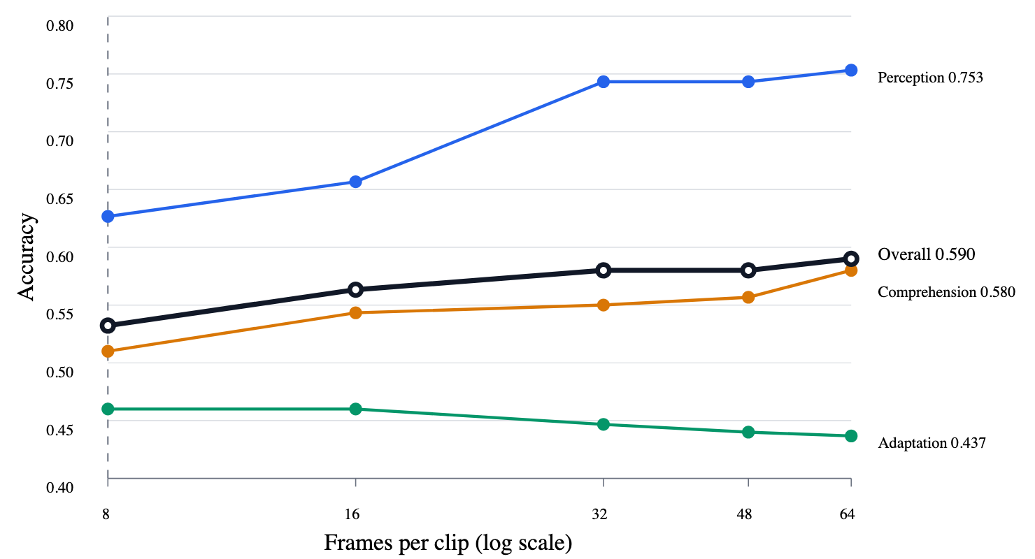
Eight frames is not much. The paper's own sweep (its Figure 2) shows Video-MMMU rising from 0.5322 at 8 frames to 0.5800 at 32 and 0.5900 at 64. The v0 headline used 64; v1's wrapper caps every input at 8 "as in training". Whatever frame count produced v1's 0.646 on the card is not stated.
6,656 numbers, every time
v1 returns a (n, 6656) float32 tensor. That is 26,624 bytes a vector, about 26.6 GB for a million documents before any index, against 3,072 bytes for a 768-dimensional model. There is no Matryoshka training mentioned anywhere: no truncation guidance, no smaller dimension, and a square head with no reason to front-load information. You can quantise the vectors yourself; whether the ranking survives truncation is untested.
Putting the options in the question
The weakness of a bi-encoder on multiple choice is easy to see in an MMLU question the paper quotes: options B and C are "red, oxidative, fast contracting" and "red, oxidative, slow contracting". The request embedding cannot know that the only word that matters is the one that differs, because it never sees the options. The candidate embeddings cannot know which property the question is asking about.
The paper's fix is blunt: when the option set is small, list it in the request. The last token then reads the alternatives and can encode which distinction the question hinges on. Training drops the list from a random fraction of closed-set rows, so the model still produces a usable request embedding when there is no list, which is the retrieval case.
The ablations make it the largest single lever in the paper. Table 3: MMLU goes from 0.5645 without the list to 0.7456 with it, +0.1811; MMMU +0.0754. Table 4 then varies the candidate side with the list present. Candidates as bare letters ("C") score 0.6512 on MMLU, far above the 0.25 of chance, which means the model is resolving a pointer: "C" carries no content, but the request embedding learned what C was. Letter plus text ("C. red, oxidative, slow contracting.") is best at 0.7767. Shuffling option order across 10 runs moves MMLU by a standard deviation of at most 0.003. The options are still listed in order, with letters, inside the request, so position could have mattered; on the paper's measurement it barely does, which is not what constrained decoders are known for.
So "decision support" is a bi-encoder doing what a cross-encoder does, by stapling the candidate list onto the request. It works for 2 to 26 options. It cannot work for a million, which is why the same model has to keep a list-free mode.
A decision is a retrieval with a short corpus
v1's wrapper has three calls. encode and retrieve are what any embedding model offers. decide is new, and it speaks the request format of Jev, TypeSafe's decision model:
result = model.decide(
    {"query": "used iphone 15"},
    {
        "shopping": {"type": "noul", "instructions": "Is the user shopping for a product?"},
        "topic": {"type": "choice", "instructions": "Which topic is the query about?",
                  "criteria": {"electronics": "", "food": "", "travel": "", "other": ""}},
    },
)
Each question becomes one closed-set row. The query is the state (a string as is, or json.dumps of an object), a blank line, Task: and the question, then Options: No, Yes or the choice keys. Each option becomes a candidate, embedded once and cached, with the instruction Option for the task: ... when the options are short labels. The answer is answer():
probs = torch.softmax(scores.double() / temperature, dim=-1)The confidence is 1 minus the entropy of those probabilities divided by , and a score question (an ordinal scale) reports the expected level index rather than the argmax. On the card's own example, "used iphone 15" gets "true" with probability 0.984 and confidence 0.881. Those two numbers are consistent with each other: two options at 0.984 and 0.016 have entropy 0.082 nats, and , within the card's rounding.
The widget works backwards from the gallery Meta published. The gallery prints probabilities; at , the cosine gap between two options is . On the ChartQA example the model picks "105.4" over "106.4" with probabilities 0.8087 and 0.0971, which is a cosine gap of 0.0424 between two embeddings of 6,656 numbers each. Everything this model decides, it decides on differences in the second decimal place of a cosine.
Two consequences follow, and both matter if you put this behind an agent.
First, the temperature changes how sure the model sounds, never what it answers. The argmax of a softmax does not move with . The wrapper's calibrate(answers, labels) fits on labelled data by grid search over 301 values from 0.001 to 1, minimising negative log-likelihood. That is ordinary temperature scaling, and it is the right tool for a threshold; it will not make a single answer more accurate.
Second, the options never see each other on the candidate side. A decision model built as a bi-encoder inherits that limit by construction, and the options-in-prompt trick only patches the request side. CLM, which the site covered in September, made the same bet with a frozen Qwen3-8B and two small heads (a softmax over 100 × cosine, so a temperature of 0.01); MetaEncoder makes it with the whole 28B backbone fine-tuned and a natural-language interface instead of a schema. Both get their speed from the same place: option embeddings are cached, so a question with a fixed option set costs one forward pass.
For where a decision model belongs at all, the site's procedure applies unchanged. The gate this model fails by design is the one about options that depend on each other ("none of the above", mutually exclusive labels), because each option is embedded alone.
The numbers behind "SOTA"
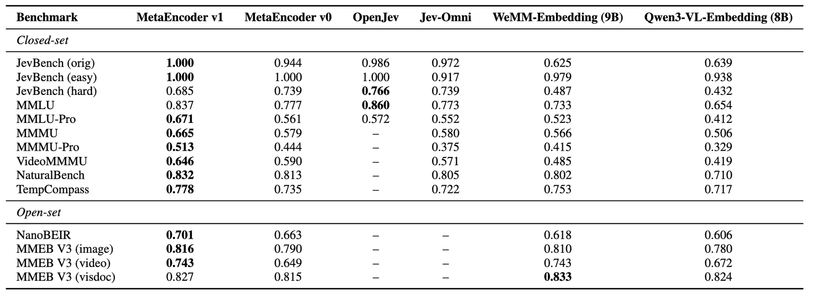
The paper describes v0, and its Table 2 matches the v0 column above to three decimals. v1's evidence is this one picture. Read row by row:
Retrieval, the four open-set rows, against WeMM-Embedding 9B (the MMEB-V3 leader the paper names). NanoBEIR, a clear win: 0.701 to 0.618. MMEB-V3 image, 0.816 to 0.810, a gap of six thousandths. MMEB-V3 video, 0.743 to 0.743: a tie, printed with only v1 in bold. MMEB-V3 visual documents, 0.827 to 0.833: a loss, which the table does bold correctly. Against Qwen3-VL-Embedding 8B, v1 is ahead on all four. Neither the card nor the paper compares against SigLIP 2 or Meta's own Perception Encoder, so how it stands against two-tower models is not something these tables can say. That is "SOTA" on one text benchmark and parity on multimodal retrieval, from a model about three times WeMM's size. The paper's own word for v0 was "near-SOTA", which was the accurate one.
v0 to v1. The gains are real on the card's terms: MMLU 0.777 to 0.837, MMMU 0.579 to 0.665, MMEB-V3 video 0.649 to 0.743. But JevBench's hard split goes the other way, 0.739 to 0.685. That split has 111 items, so v0 got 82 right and v1 gets 76, while OpenJev 27B gets 85. The original split went from 0.944 to 1.000, 72 of 72, and easy stayed at 48 of 48; on a public set whose items have been a development target for two months (the site's reproduction piece documents at least one entrant tuning on it), two perfect scores are the least informative numbers in the table. Two rows from v0's table are gone in v1's: "Jev Intelligence" and ImaJev, the multimodal decision benchmark. MMLU-Pro, MMMU-Pro and a Jev-Omni column are new. The v0 column's MMMU-Pro, 0.444, matches no encoder figure in the paper (Tables 3, 4 and 6 give the encoder between 0.3503 and 0.5601, depending on options and rendering). The nearest number in the paper is 0.4441, which Table 6 gives for the constrained-decoder baseline. That is either a coincidence or a copied cell, and I cannot tell which from the outside.
The evaluation repo disagrees with the paper. meta-encoder-eval exists to reproduce v0's table, and compare.py passes a suite within 0.005 of reference_scores.json. That file's MMEB-V3 video score is 0.6046, the mean of its 18 tasks; the paper and the repo's own README image say 0.6486. Its MMLU is 0.7541 (the unweighted mean of 57 subjects; weighted by the 14,042 test questions it is 0.7395 on my arithmetic), against 0.7767 in the paper's Table 2. A reader who runs the repo and matches its reference has not reproduced the paper.
Some settings were chosen on test data. The eval README says so plainly about Video-MMMU: "The frame count was set after a sweep on the test set itself (Video-MMMU has no development split)". The NanoBEIR prompt gives the e5-mistral instruction to the seven subsets "with a counterpart in training" and none to the other six. The paper's own appendix, meanwhile, lists a query instruction for all thirteen NanoBEIR subsets, so the paper and the repo do not even describe the same protocol. Neither choice is hidden, and neither is what a held-out number means.
Where one vector runs out
The paper's best section is the one where it argues against its own model. It compares MetaEncoder with its own base, Muse Glimmer, used as a constrained decoder: same prompt, all options listed, logits read off the letters. On MMLU they tie, 0.7740 against 0.7743. On MMMU the encoder wins, 0.5730 to 0.4962. The paper traces that to the decoder not wanting to answer with a bare letter: the letter tokens carry 0.8679 of its probability mass on MMLU but only 0.7424 on MMMU.
Then it lets the decoder think.
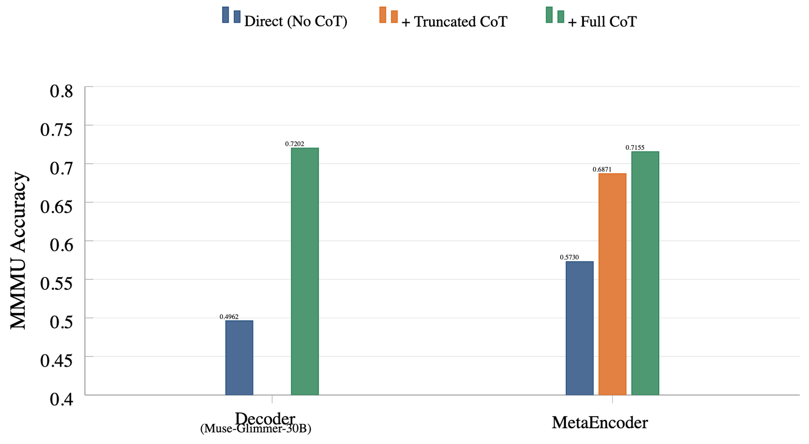
Unconstrained, Muse Glimmer reaches 0.7202 on MMMU. Fed that reasoning as extra context, MetaEncoder reaches 0.7155; with the answer label removed from the trace (it appeared in 93.7% of them), 0.6871. The paper draws the conclusion against itself: the bottleneck is "whether intermediate reasoning is provided", not how the candidates are scored. A single forward pass, however large, does what an LLM does without thinking, and the gap of about 0.2 on MMMU that the paper names is the size of that.
For retrieval that is fine; nobody wants their search index to reason. For decisions it means MetaEncoder is a fast first pass that is good at reading, perception and classification, as the paper says, and that something has to escalate the hard rows. In an agent that drafts project documents from meeting notes, which is the kind of thing I build on Kaël, "is this note about a change request?" is a question it should answer well. "Does this change conflict with a clause in the contract?" is a reasoning question wearing a classification costume, and the paper's own figure says to route it to something that can think first.
What it costs, and the missing licence
Every embedding costs a forward pass through 28.4B parameters. That is about 38 times EmbeddingGemma 2's 744M per token, and indexing is where an embedding model spends most of its life. The eval README budgets one full bf16 copy per 80 GB GPU, "about 62 GB", and eight GPUs for the benchmark run. Images keep their native resolution up to 4,096 tokens each, and inputs are never truncated because truncation would cut off the pooled token; the wrapper warns past 16,384 tokens, the longest training sequence. A single A4 scan at full resolution is several thousand tokens through a 52-layer, 6,656-wide decoder. Plan on a datacenter GPU per query stream, not a CPU.
Then the licence. v0 says Apache-2.0, inherited from Muse Glimmer, plus Muse Glimmer's usage policy and a NOTICE. v1, the release everyone is linking, has no LICENSE, no NOTICE, no usage policy and no license: field in its card; I checked that the files return 404. With no licence, the default is that you have no grant to use the weights. It is probably an oversight, given v0, but "probably" is not a licence.
Where I land
The architecture is the interesting thing here, and it holds up: one large decoder, last-token pooling, one-directional InfoNCE with task-dependent negatives, and a decision API that is retrieval over a short corpus with the candidates written into the question. The paper is unusually candid about where that design stops, and the CoT experiment is the most useful result in it.
The release is weaker than the architecture. "SOTA retrieval" is one win, one near-tie, one tie and one loss against a model a third the size. The paper is for a different checkpoint, the repo meant to reproduce it disagrees with it by 4.4 points on video, and the new checkpoint has no licence and no evaluation artefacts beyond a PNG. If you need multimodal retrieval today, a 9B model matches it at a third of the cost. If you want to see how far a bi-encoder can go as a decision maker, this is the right paper to read, and v0, which is licensed, is the right checkpoint to try.
How I checked: I read the paper (arXiv HTML), both model cards, v1's config.json, processor_config.json, chat_template.jinja and modeling_metaencoder.py, and the safetensors headers of all twelve v1 files by HTTP range request; the base model's model.safetensors.index.json for lm_head; v0's README (its weights and code are gated); the eval repo at ecc7792, including reference_scores.json and compare.py; and the Space's gallery.json. Parameter counts, the MMLU weighted mean and the cosine gaps are my arithmetic on those files. I did not run the model: 57 GB of weights did not fit this task. Every v1 benchmark number is the card's.