2026-11-13 · 28 min · speech · audio · tts · tokenization · liquid-ai · on-device
A 2:44 narrated explainer, drawn in code. Every number and picture in it is this article's own; the sources are below.
› transcript
Next-token prediction scales because text comes from a discrete, fixed vocabulary. Audio doesn't. So turn the waveform into tokens, train on the tokens, and turn them back into sound. Hi, I'm Fintan! A language model predicts integers. Speech is twenty-four thousand real numbers a second. A codec sits in between. Every neural codec has three parts. An encoder squeezes time into a few vectors a second. A quantiser turns each vector into integers. A decoder turns integers back into sound. The old way is residual quantisation. Codebook one picks the nearest vector. Codebook two quantises what is left over, and so on, each correction smaller than the last. Here is a toy in two dimensions. Each code is a correction to the codes before it, and the path closes in on the point. Now let the model get code one slightly wrong. The later codes still describe the old leftover, so the whole path misses. Grouped scalar quantisation throws the codebooks away. Each of four numbers is rounded to its own grid of levels. Twelve groups make twelve tokens. A wrong code for one group moves one number by one step. The others are still right. Liquid's own figure. Four numbers, with eight, seven, six and six levels. Together they pick one of two thousand and sixteen codes. Twelve groups, twelve tokens a frame. The bill is three numbers multiplied. Twelve and a half frames a second. Twelve codes a frame, so a hundred and fifty tokens a second. About eleven bits each. Mimi with twelve codebooks lands on the same bitrate, which makes it a fair rival. Inside, the encoder starts from a spectrum, seventy-five a second, stacks six into one, and runs an eight-block LFM3 stack. The decoder runs the same stack, then predicts a spectrum and lets an inverse FFT make the samples. No learned upsampling at all. On Liquid's eight test sets it has the best perceptual quality score and the lowest mel distance on every one. The PESQ score goes the other way. NanoCodec wins seven of eight. And in text to speech, its tokens give the lowest error rate on four sets of eight. That is the better experiment: the same backbone, data and compute, only the codec changed. Mimi doubles the error rate. A speech codec's real customer is the language model that has to predict its tokens. Round instead of chain, keep the bitrate, decode the spectrum. Thanks for watching! Every source is in the full article. I'm Fintan. Bye!
Why read this
Notabletop 60%Neural audio codecs from first principles, LiquidCodec's code and header against its claims, RVQ and FSQ side by side, and the codec bitrate maths.
- Original analysis
- Runs on a laptop CPU
- Widely used
Speech & audioCustom licencePractitioner model
How this was scored
- Is it new?
- 1 of 3: An incremental tweak
- Can I trust it?
- 2 of 3: Measures key facts from files, code or configs
- Can I run it?
- 2 of 3: Open code or weights with real limits
- Will I understand it?
- 2 of 3: Mechanism from first principles with figures
- Can I act on it?
- 2 of 3: A concrete recipe, numbers or comparison
- Will it last?
- 2 of 3: A reference for a year or more
- Does it affect many?
- 2 of 3: A widely used model, tool or lab release
- Only here?
- 2 of 3: A teardown or measurement few others did
Score 66 of 100, ranked 263 of 740 rated articles. Each question is answered 0–3 by hand, and a 3 is rare. How articles are scored
On 12 November Liquid AI announced LiquidCodec, "our ~74M-parameter streaming audio codec powering LFM3-Audio-2B and LFM3-Omni-2B", and built it, in the thread's words, around "tokens that are easy to predict and fast conversion back into speech". Six hours later Alexander Amini, Liquid's co-founder, put the reason in two sentences: "LLM next-token prediction scales because text comes from a discrete, fixed vocabulary. Audio doesn't - it's a continuous waveform signal." His post is the whole idea in eight seconds:
The codec sets how many steps a second a speech model takes, what it may forget about the voice, and how fast a reply becomes sound on a phone. Liquid wrote an engineering blog with its architecture, training recipe and results, and published the weights and modelling code on Hugging Face. I read both, read config.json, the two modelling files and the licence, and pulled the 22,832-byte safetensors header with two HTTP range requests. I did not run the model. The site already ran this exact codec on CPU in the LFM3-Omni WebGPU piece; I lean on those measurements where they apply and say so.
- architecture
- LiquidCodecModel
- task
- feature-extraction
- library
- transformers
- license
- other
- safetensors
- 1 shard
- largest file
- 147.1 MB
- files
- 9
- downloads
- 9.8K
- likes
- 70
- languages
- en, zh, de, fr, ja, ko
repo last modified 2026-11-12
Why a language model cannot eat a waveform
A language model is a classifier run in a loop: a probability for every entry of a fixed vocabulary, one sampled, fed back in. Text suits it because text is already discrete and slow, a few tokens a second of speech.
Audio is the opposite on both counts. A 24 kHz recording is 24,000 real numbers a second. You can force it into a vocabulary (WaveNet quantised each sample to 256 μ-law levels and predicted them one at a time), but then a single second of speech is 24,000 sequential steps, and a ten-second reply is a sequence longer than most text contexts. And no single sample means anything; words, voice and mood live in patterns tens of milliseconds long.
So every speech language model puts a learned compressor in front of the transformer, turning audio into a short vector a few dozen times a second or fewer, and a decompressor behind it. What the vectors look like splits the field in two.
- Discrete tokens. Quantise each vector into integers from fixed codebooks. The language model then predicts integers with the softmax it already has. Moshi, Mimi, EnCodec, X-Codec 2, NanoCodec and LiquidCodec are this camp.
- Continuous latents. Keep the vector real-valued and train a small sampler (diffusion or flow matching) to generate it from the language model's hidden state. Today's other speech article on this site, Haru-4B, is this camp: 64 real numbers every 133 ms from VibeVoice's tokenizer, sampled by a one-step MeanFlow head.
LiquidCodec is a firm vote for the first camp, built to remove the costs that push people toward the second.
Why Liquid stopped borrowing Mimi
Liquid's audio models have changed codec set-ups in each of three generations, and the blog is candid about why. LFM2-Audio-1.5B used Kyutai's Mimi whole, for its "high compression (1.1 kbps bitrate) and a low parameter count (~96M)". LFM2.5-Audio-1.5B kept Mimi's tokenizer and replaced only the detokenizer, which made decoding 8 times faster. For LFM3 they built both halves, because, in the thread's words, "keeping Mimi's tokenizer meant we were still limited by its token quality and architectural choices." Leonie Monigatti's post from Liquid's team puts it as plainly: the earlier models' third-party tokenizer's "token quality and design choices started to limit us". Her post carries the blog's pipeline figure, which is the shape of everything that follows:
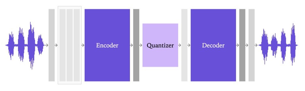
The decoder they had was already fast. The tokenizer, the part the language model learns to imitate, was the part they could not change.
Encoder, quantiser, decoder
The modern neural codec has three parts, and Liquid's own animation of its pipeline names them:
The encoder reduces time. In SoundStream and EnCodec strided convolutions multiply up to 320 (8, 5, 4 and 2 in facebook/encodec_24khz), so 24 kHz audio becomes 75 vectors a second. Mimi and NVIDIA's NanoCodec go down to 12.5, one every 80 ms.
The quantiser turns each vector into integers; it gets the next two sections.
The decoder turns codes back into samples. In the SoundStream lineage it is the encoder run backwards, transposed convolutions upsampling to 24,000 numbers a second, and its last layers are expensive because they run at the full sample rate. The cheaper alternative, popularised by the Vocos vocoder, predicts a short-time spectrum and lets a fixed inverse FFT make the samples. LiquidCodec does that.
Training has two kinds of loss. Reconstruction losses (an L1 on the waveform, mel distances at several resolutions) get the audio right on average and wrong in texture, because the average of many plausible fine structures is a smeared one. Adversarial losses fix the texture: discriminators that look at the waveform folded at prime periods, at multi-band spectra, or at a speech model's features learn to tell real from reconstructed, and the codec learns to fool them. DAC is built on this mix, and NanoCodec's model card lists all three kinds of discriminator.
One more distinction matters for language modelling. Acoustic tokens are whatever minimises reconstruction error; they encode the speaker, the room and the microphone as eagerly as the words. Semantic tokens come from a self-supervised speech model (HuBERT, WavLM, w2v-BERT) and encode mostly content. Codecs built for speech LMs often blend the two. Mimi distils WavLM into its first codebook, as the Moshi paper describes; X-Codec 2's config carries a full facebook/w2v-bert-2.0 as its semantic_model_config. Liquid's blog describes only waveform, spectral and adversarial losses and no semantic teacher; without training code I cannot rule one out, but nothing points to one. Keep that in mind when it comes to "easy to predict".
Residual codebooks, and why the codes depend on each other
The quantiser everyone used until recently is the residual vector quantiser (RVQ), which goes back to multistage vector quantisation for speech coding in 1982 and arrived in neural codecs with SoundStream. Take the encoder's vector . Codebook 1 is a learned list of, say, 2,048 vectors; pick the one nearest to and call it . What is left, , is quantised with codebook 2, and so on:
Each stage spends bits refining what the previous ones missed. Mimi has 2,048 entries per codebook (11 bits) and up to 32 codebooks; Moshi uses eight of them, 8 × 11 × 12.5 = 1,100 bits a second, the 1.1 kbps Liquid's blog quotes. Liquid's own animation of the scheme, from the blog's Figure 2, shows the residual shrinking stage by stage:
RVQ compresses well. The trouble is for whatever generates the codes. Code 2 means "this correction, given that code 1 was what it was". Change code 1 and the right code 2 changes with it. A model can predict a frame's codes one after another, each conditioned on the ones before, which is what Moshi's small "depth transformer" does: eight extra sequential steps per 80 ms frame. Or it can predict them in parallel and accept that a wrong code 1 leaves the others correcting a residual that no longer exists.
In two dimensions: drag the point, add codebooks, then tell the toy the model picked the runner-up for code 1.
With RVQ the dashed path (later codes kept as they were) lands far from the point, often farther than the first code alone would have; the solid path (later codes re-chosen for the new residual) recovers, but only because it was allowed to look at code 1 first. That is the dependency Liquid's thread means when it says RVQ "creates strong dependencies between codebooks", and its blog when it says each codebook "strongly influences its successor".
Finite scalar quantisation: just round
Finite scalar quantisation (FSQ), from Google in 2023, throws the codebooks away. Project the vector down to a handful of dimensions, squash each dimension into a bounded range, and round it to one of evenly spaced levels. The "codebook" is implicit: every combination of levels is a code, so a group of dimensions with levels has codes. Nothing in the quantiser is learned, so nothing collapses and no dead entries need reseeding, which is the FSQ paper's pitch. Gradients pass the rounding by the straight-through estimator.
Grouped FSQ (GFSQ, from Fish-Speech) splits the vector into several groups and gives each its own FSQ. Each group yields one integer, and the groups describe disjoint coordinates, so no group's code changes meaning when another's does. In the toy above, that is the right-hand plane: a wrong code moves the point along one axis by one step, and the other code is still right.
LiquidCodec's quantiser is short enough to read whole. From modeling_liquid_codec.py in the Hugging Face repo:
# LiquidAI/Liquid-Codec, modeling_liquid_codec.py, LiquidCodecQuantizer (abridged)
latents = self.project_in(latents.movedim(1, -1).contiguous()).float()   # 256 -> 48
latents = latents.reshape(*latents.shape[:-1], self.num_codebooks, self.codebook_dim)  # 12 x 4
half_width = self.levels // 2
codes = self._bound(latents).round() / half_width
indices = ((codes * half_width + half_width) * self.basis).sum(-1).round().long()
The numbers come from config.json: quantizer_dim 256, n_q 12, fsq_levels [8, 7, 6, 6]. A linear layer maps the encoder's 256-dimensional latent to 48 numbers, which are cut into 12 groups of 4. _bound squashes each number with a shifted tanh into the range of its levels (the shift puts an even number of levels symmetric about zero), and rounding picks a level. The four level indices of a group are combined in mixed radix (basis is 1, 8, 56, 336) into one integer below 8 × 7 × 6 × 6 = 2,016. Twelve integers per frame, each from a vocabulary of 2,016. The blog's Figure 3 animates one group:
Those levels are not new: NVIDIA's NanoCodec card lists [8, 7, 6, 6] and 2,016 codes for its 1.78 kbps model, with 13 codebooks. What Liquid changed is around the quantiser.
One caution on "independent". The twelve groups are slices of one projection of one encoder state, so a frame's codes are still statistically correlated. What GFSQ removes is the structural dependency, a code's meaning defined relative to an earlier code. The model card goes further than the blog and says GFSQ "produces codebooks with no sequential dependencies, so speech models can predict all codebooks of a frame in parallel". In practice LFM3-Omni does not predict all twelve at once: its config's maskgit_schedule is [4, 4, 4], three passes of a small depth decoder revealing four codes each, as the WebGPU piece found. That is a quarter of the passes of a one-code-at-a-time decoder.
The bill: frame rate times codebooks
A codec's bitrate is three numbers multiplied: frames per second, codes per frame, and bits per code.
That is about 1,647 bits a second, which the model card rounds to "≈ 1.65 kbps". Against 16-bit PCM at 24 kHz, 384,000 bits a second, that is a compression of about 233 times. The more useful number for a language model is the code rate: 12.5 × 12 = 150 integers a second, 9,000 a minute.
If every code were one backbone step, a minute of speech would be 9,000 positions and 9,000 sequential passes. The standard trick, Moshi's, sums a frame's code embeddings into one vector, takes one backbone step per frame (750 a minute), and lets a small decoder produce the frame's codes. The calculator works through the trade with each codec's published configuration.
The presets make the comparison easier to read. Liquid's comparison is at matched bitrate where it counts: Mimi at 12 codebooks is 12 × 11 × 12.5 = 1,650 bits a second, within 4 bits a second of LiquidCodec. It is not matched everywhere. NanoCodec is 1.78 kbps at 22,050 Hz, a little richer. X-Codec 2 is 800 bits a second (one code from 65,536, 50 times a second, from 16 kHz audio), half the bits and two-thirds of the bandwidth, so its lower reconstruction scores are partly its operating point. And the low frame rate is a deliberate inheritance. The blog says Liquid "kept the same frame rate of 12.5 Hz" to preserve the efficiency of its previous audio models, which used Mimi.
Inside LiquidCodec
Liquid's architecture figure from the thread matches the code:
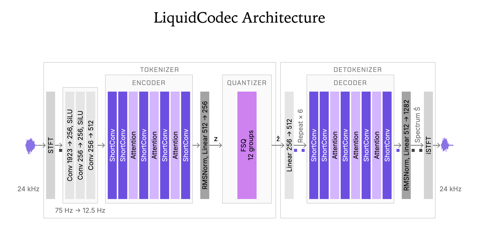
Following a frame through modeling_liquid_codec.py:
- STFT. A 1,280-sample Hann window every 320 samples: 75 spectra a second of 641 bins. Each bin contributes
log1pof its magnitude and the cosine and sine of its phase, which is the "1923" in the figure, 3 × 641. - Convolutions. A 1×1 convolution to 256 channels, a width-3 convolution padded on the left only (causal), and a convolution with kernel and stride 6 that merges six spectra into one 512-dimensional vector. 75 Hz becomes 12.5 Hz here, before the transformer.
- Encoder. An LFM3 stack from Liquid's own LLM family (taken apart in the LFM3 piece): 8 layers of width 512, with attention as the third, fifth and seventh (8 query heads, 2 key-value heads of 64 dimensions) and gated short convolutions of width 7 everywhere else. Attention is causal and unwindowed, so the encoder can look back over the whole clip.
- Quantiser. A linear layer to 256, then the FSQ above.
- Decoder. Codes back to 48 numbers, a linear layer to 256 and another to 512, then each frame's vector is repeated six times (
F.interpolatewithnearest-exact) to get back to 75 Hz. The same 8-layer LFM3 stack runs at that rate with a sliding attention window of 30 positions, which is 400 ms. - Spectrum and inverse STFT. A linear layer maps each 512-dimensional state to 1,282 numbers: a log-magnitude and a phase angle for each of the 641 bins. An inverse FFT and overlap-add make the samples.
Step 6 is the speed trick: no learned upsampling, nothing learned above 75 positions a second, and the last 320-fold expansion is an FFT. It also explains why the WebGPU piece found a round trip that kept the spectrum (10.6 dB STFT-magnitude SNR) and not the waveform (−0.4 dB): a decoder that predicts its own phase owes you a signal that sounds the same, not one that lines up sample for sample.
The thread's second picture shows the block pattern that both halves share:
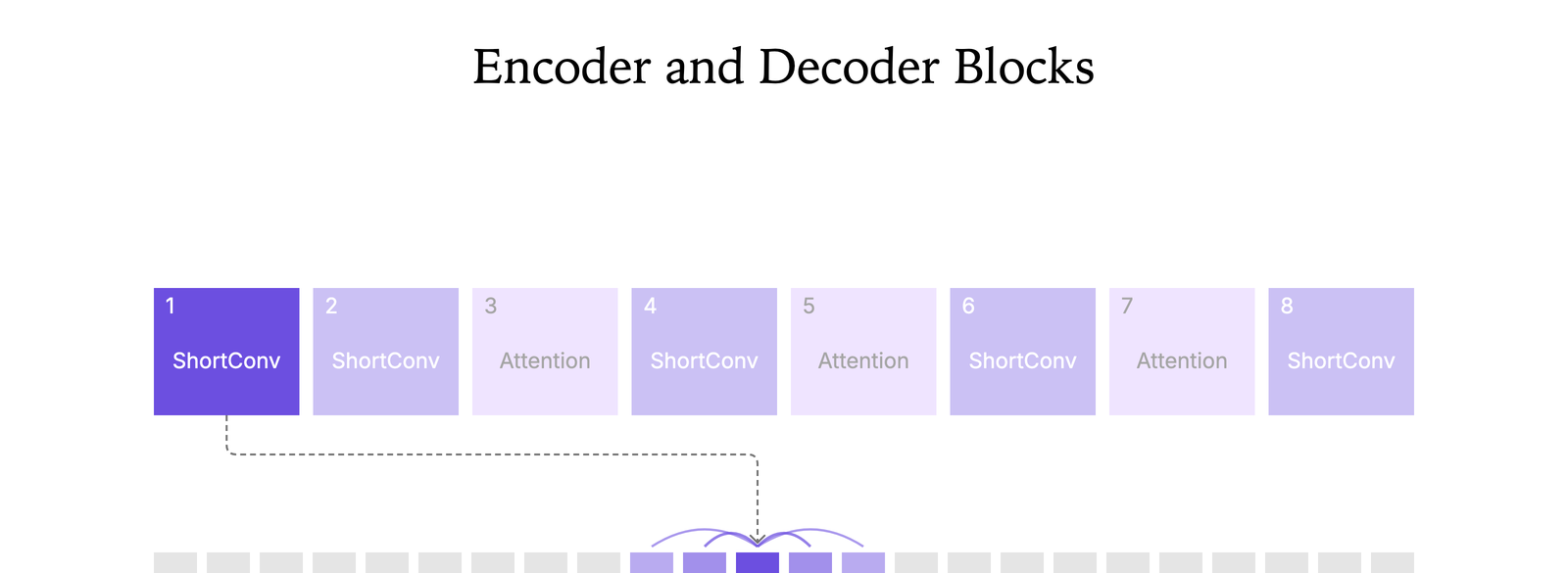
That caption needs one correction, which the code settles: Lfm3ShortConv pads by kernel_size - 1 and keeps the first seq_len outputs, so a frame reads itself and the six before it, never after.
Where the 74 million parameters are. The header has 73,559,090 values, all BF16 except a 1,280-entry float32 buffer that is the inverse STFT's window. Grouped by module:
| Part | Parameters |
|---|---|
| STFT front-end convolutions | 1,476,352 |
| Encoder LFM3 (8 layers) | 35,568,000 |
| Encoder to quantiser, projection in | 143,664 |
| Tokenizer side | 37,188,016 |
| Projection out, quantiser to decoder | 144,128 |
| Decoder LFM3 (8 layers) | 35,568,000 |
| Linear to spectrum, window buffer | 658,946 |
| Detokenizer side | 36,371,074 |
The two LFM3 stacks are identical to the parameter, which is what "exactly symmetric" means in the blog. They are not symmetric in work: the decoder's stack runs six times per frame, the encoder's once.
What "streaming" buys and costs
On the way in, the encoder needs a whole 80 ms frame of 1,920 samples before it can emit that frame's twelve codes, and a little more: the STFT pads by 480 samples, so the last of a frame's six analysis windows reaches 20 ms past the frame's end. Offline, the code fills that with a reflection of the signal. The released code also has no streaming encoder. encode() takes a whole waveform, and LiquidCodecStreamingCache exists only for decode(), so the card's "Streaming encoding and decoding" is true of the design and half true of the download.
On the way out, decoding is properly incremental. Each frame of codes produces 2,880 samples of overlap-add, and the cache holds back the trailing 960 until the next frame adds to them. Do the bookkeeping and after frames the decoder has released samples: 60 ms for the first frame, 80 ms for each after, with the last 20 ms of every frame waiting for the next. The cache also keeps the decoder's convolution buffers and its 30-position attention window, so each frame is one pass over six positions. For TTS, then, the first 60 ms of audio exist as soon as the first twelve codes do; a full round trip adds the 80 ms frame plus about 20 ms at each end, before compute.
Training: no GAN first, then a GAN
The blog describes two stages. Stage one: 264,000 hours of speech in 107 languages ("web speech with audiobooks, crowd-sourced recordings, and smaller parliamentary and meeting collections"), trained only with waveform and spectral losses. That left what the blog calls "metallic" artifacts, which it attributes to reconstruction losses "averaging out" fine detail. Stage two: 55,000 hours of cleaner speech, all natively sampled at 24 kHz or above, with "adversarial critics that examine waveform patterns, spectral detail, and speech features". The critics are not named; the description fits NanoCodec's trio, but that is my reading.
Then decoder-only quantisation-aware training, so the decoder survives 4-bit weights. The blog says Q4_0 "can also reduce its decoder footprint by a factor of 3.5". The arithmetic agrees: llama.cpp's Q4_0 stores 32 weights in 18 bytes, 4.5 bits a weight, and 16 / 4.5 is 3.56. The quantised decoders are not in this repo; the card says they ship inside the LFM3-Audio-2B-GGUF and LFM3-Omni-2B-GGUF files.
Neither the blog nor the card links any training code, and the data mix is described only as above. The weights are under the LFM Open License v1.0, which grants Apache-style rights with one condition in section 5: commercial use is licensed only to entities under 10 million US dollars of annual revenue.
What the results table says, and what it leaves out
Liquid evaluated two things, and the second is the one that matters.
Reconstruction. Encode a recording, decode it, compare with the original, on eight test sets: LibriSpeech test-clean, Seed-TTS English and Mandarin, and FLEURS in German, French, Mandarin, Japanese and Korean. The metrics are SQMOS (a predicted quality score), wideband PESQ, mel distance, speaker similarity (SECS with ECAPA2 embeddings), ViSQOL, and the character error rate of a recogniser on the reconstruction. LibriSpeech, from the blog's table:
| Codec | PESQ (WB) ↑ | Mel dist. ↓ | SECS ↑ | ViSQOL ↑ | Recon. CER % ↓ | TTS WER % ↓ | TTS UTMOSv2 ↑ |
|---|---|---|---|---|---|---|---|
| LiquidCodec BF16 | 2.640 | 0.120 | 0.785 | 4.319 | 0.89 | 3.15 | 3.31 |
| LiquidCodec Q4_0 | 2.577 | 0.121 | 0.781 | 4.292 | 0.89 | 3.18 | 3.22 |
| X-Codec 2 | 2.434 | 0.123 | 0.754 | 4.119 | 0.88 | 4.19 | 3.27 |
| NanoCodec | 2.942 | 0.122 | 0.836 | 4.219 | 0.76 | 3.32 | 3.19 |
| Mimi (12 codebooks) | 2.615 | 0.160 | 0.714 | 4.031 | 0.87 | 6.27 | 2.89 |
I tallied each metric's winner over all eight test sets (the card's copy of the table matches the blog's), leaving out the Q4_0 row. LiquidCodec has the best ViSQOL and the lowest mel distance on all eight, exactly as claimed. It does not lead everything. NanoCodec has the best PESQ on seven of eight (LiquidCodec takes Korean) and the lowest reconstruction CER on seven of eight. Speaker similarity is split, NanoCodec four, LiquidCodec three, X-Codec 2 one. The blog's phrase for this, "competitive on the other metrics", is fair. NanoCodec's card also says its encoder is non-causal, which LiquidCodec's is not; that is a real handicap for a streaming codec to carry into the comparison.
Speech generation. This is the better experiment. Liquid trained four TTS models, one per codec, with everything else fixed: the same 101,000 hours in six languages, a backbone initialised from LFM3-1.7B, "a six-layer, 1,024-dim autoregressive depth decoder to predict the codebooks within each audio frame", identical batches in identical order and the same compute. Only the token embeddings and output heads differ. Each model then reads text with no voice prompt, three seeds. LiquidCodec's models have the highest UTMOSv2 naturalness on all eight sets, and the lowest WER or CER on four (both English sets, Seed-TTS Mandarin, and German). Mimi at matched bitrate trails: double the WER on LibriSpeech. Liquid says a repeat with a Qwen3-1.7B backbone gave consistent results; that table is not published.
Before quoting it, know what it does and does not test.
- It does not test the parallel prediction GFSQ was chosen for. All four TTS models use the same autoregressive depth decoder, one code after another. So the result says LiquidCodec's tokens are easier to learn even when predicted sequentially, which is a stronger and different claim from "GFSQ enables parallel prediction". The MaskGIT path that LFM3-Omni actually uses is not compared against anything.
- X-Codec 2 is an odd member. With one code per frame its depth decoder has nothing to do, and unless frames were stacked (the blog does not say) the backbone runs at 50 Hz instead of 12.5. That tests a different design, not a worse quantiser.
- The noise floor is not stated. The Q4_0 row differs from BF16 only in the decoder. On five sets their TTS WERs are within 0.08 points; on three FLEURS sets the Q4_0 row is lower by 1.65 (French, 5.26 against 6.91), 1.65 (Korean, 6.71 against 8.36) and 0.98 (Mandarin). The blog does not explain the swing, and neither can I. Counted on the Q4_0 row, LiquidCodec still wins four of eight, but a different four: German drops out and French comes in. I read the WER result as a close race rather than a win.
What "easy to predict" means. A code from 2,016 values carries at most bits, so a frame carries at most about 132 bits. If a code is close to a coin toss given everything before it, the language model has to model 11 bits of near-noise per code; if its variation is predictable from the text and the previous frames, cross-entropy is low and sampling is stable. The measurements that would show it are the codes' empirical entropy (how evenly the 2,016 values are used) and their conditional entropy under a trained model (the TTS models' loss per code). Liquid publishes neither, nor any codebook-usage figure, and without running the model I cannot measure them. What it does publish is the downstream outcome: the same model, trained the same way, makes more natural speech from LiquidCodec's tokens. That is the evidence that matters most, and it is one experiment.
One example, measured. The blog includes a 62.5-second original and its LiquidCodec reconstruction, both 24 kHz float WAV, which I compared in numpy. Waveform SNR is −2.5 dB, as expected for a codec that predicts its own phase. STFT-magnitude SNR is 8.2 dB and the log-spectral distance is 3.1 dB. The energy in each band (below 1 kHz, 1-4 kHz, 4-8 kHz, 8-12 kHz) is within 0.7 dB of the original, so nothing is band-limited away. It is one clip chosen by Liquid; it shows the codec is not cheating on bandwidth, not that it is good on your audio.
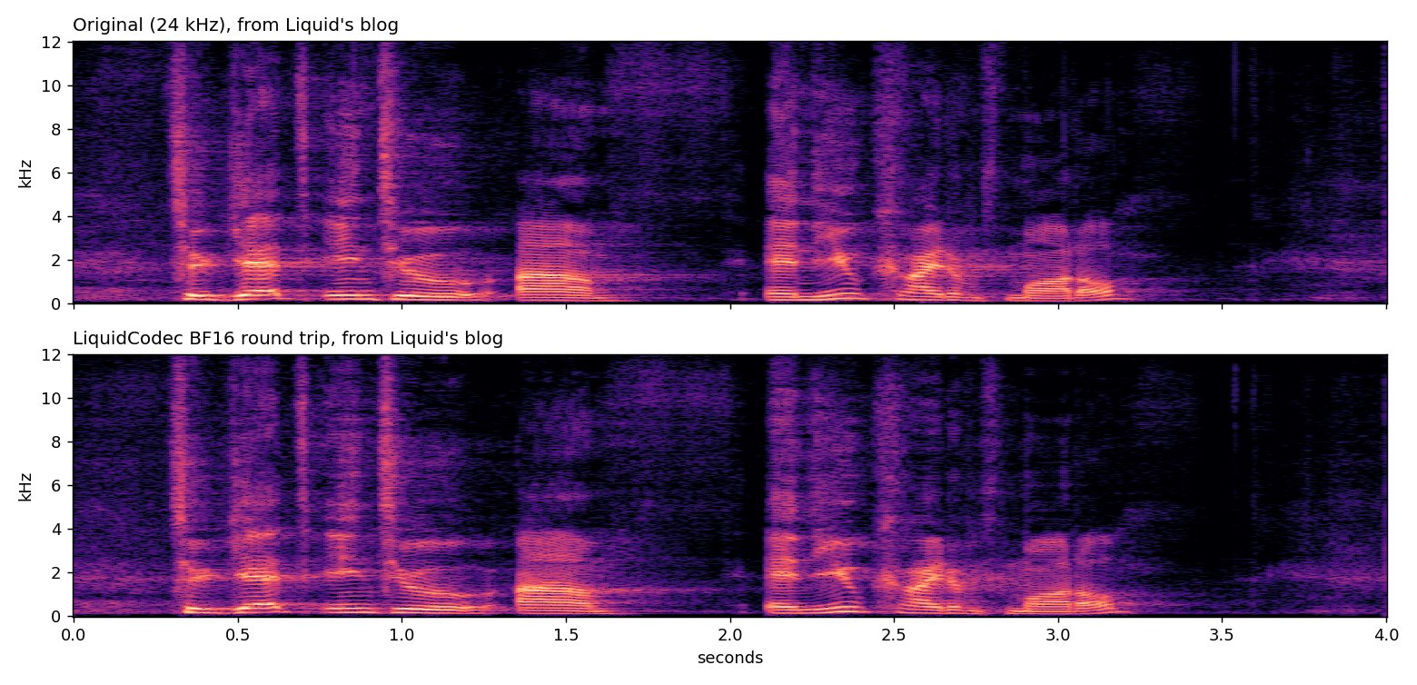
Is it really that fast?
The headline: on one CPU thread of an Apple M4 Max at FP32, about 361 times real time to encode and 87 times to decode. The blog's Table 2 gives real-time factors: 0.0028 ± 0.0001 to encode and 0.0115 ± 0.0001 to decode. The reciprocals are 357 and 87; 361 sits inside the error bar. For comparison, Mimi's RTFs in the same table are 0.0361 and 0.0329, NanoCodec's 0.2145 and 0.2543.
Per 80 ms frame that is 0.22 ms to encode and 0.92 ms to decode. By my count the encoder does about 80 million floating-point operations a frame (its 35.6M-parameter stack once, plus the front end) and the decoder about 435 million (the same stack six times). Five times the arithmetic, four times the time: a consistent pair.
The absolute rate is the surprise: about 360 billion operations a second for the encoder and 470 billion for the decoder. By my estimate one M4 performance core's NEON units peak near 140 billion FP32 operations a second, so the likely explanation is Apple's matrix unit, which Accelerate's BLAS drives from a single thread. The number is real but specific: one thread on Apple silicon is not one thread on a phone, and whole clips encoded in one call are not the frame-by-frame loop a live app runs. The WebGPU piece measured that loop for this codec in plain PyTorch on two CPU threads: 30.5 ms median per 80 ms frame.
Two camps, one problem
Put LiquidCodec next to Haru-4B and the trade is clear.
Haru uses VibeVoice's continuous tokenizer: one 64-dimensional real vector every 133 ms. Nothing is snapped to a codebook and a frame is one vector, so there is no codebook axis to generate along. The price is a sampler that is not a softmax, a one-step MeanFlow head of 363 million parameters, and a codec of 687 million, nine times LiquidCodec.
LiquidCodec keeps the softmax, so temperature, top-p, the loss and the serving stack of a text LM apply unchanged to audio codes. The costs it pays (quantisation error, a second axis of twelve codes per frame) are the ones it was designed to shrink: FSQ for a codebook that cannot collapse and whose groups do not chain, 12.5 Hz to keep the backbone's sequence short, MaskGIT passes to fill a frame in three steps rather than twelve, and a decoder small enough to run 4-bit on a phone. Elsewhere on this site, Fish Audio S2 stays discrete with ten codebooks and a four-layer fast decoder, Pocket TTS goes continuous with a one-step head, Qwen Audio 3.0 TTS predicts 12.5 Hz semantic tokens and leaves the voice to a flow-matching decoder, and PersonaPlex inherits Mimi and Moshi's depth transformer.
Neither camp has won. LiquidCodec is the most careful case for the discrete side I have seen from a lab shipping on-device models: a codec built for the LM that consumes it, at Mimi's bitrate, with a TTS experiment in which the codec is the only variable.
What I would do with it
For a speech LM that has to run on a device, LiquidCodec is the codec I would start from today. It is small (73.6M parameters, 147 MB in BF16, and by my arithmetic about 20 MB for a Q4_0 decoder), its decoder never runs a learned layer above 75 Hz, it loads in Transformers with remote code, and its token rate fits a 12.5 Hz backbone. The licence is fine for anyone under the revenue threshold and not for anyone over it.
I would not take two of its claims at face value. "Streaming encoding" needs your own incremental encoder; the released one is offline. And "easy to predict" is so far one controlled experiment, run with an autoregressive depth decoder rather than the parallel one the quantiser was chosen for, and its WER wins change membership when only the decoder changes. On reconstruction it is best on ViSQOL and mel distance and behind NanoCodec on PESQ and reconstruction CER. For a codec whose job is to be generated by a language model, that is the right trade, and Liquid made it on purpose.
How this was checked
Read: the blog, the three X threads (via the fxtwitter mirror), the Hugging Face card, config.json, both modelling files and the licence. Run by me: the safetensors header count (by range request, no weights downloaded), a script tallying the card's results table, and a numpy comparison of the blog's two WAV files. Arithmetic: bitrates, latencies and operation counts, from the config and code; the NEON peak is an estimate. Quoted: the CPU run of this codec from the WebGPU piece, and the other codecs' rates from their configs, cards and the Moshi paper. Clips 3 and 4 record the blog's animated figures in a headless browser stepped one frame at a time; clips 1 and 2 are the posts' videos without audio.