2026-11-09 · 17 min · simulation · sensors · event-cameras · lidar · thermal · blender · robotics · synthetic-data

Why read this
Notabletop 60%Ports VisionSIM's event, single-photon and iToF emulators and measures them; finds the iToF noise and bolometer lag missing from the shipped code.
- Original analysis
- A lasting reference
- A new technique
Robotics & embodiedNeeds a workstation GPUGPL-3.0-or-laterPractitioner tool
How this was scored
- Is it new?
- 2 of 3: A real new idea, method or capability
- Can I trust it?
- 2 of 3: Measures key facts from files, code or configs
- Can I run it?
- 2 of 3: Open code or weights with real limits
- Will I understand it?
- 2 of 3: Mechanism from first principles with figures
- Can I act on it?
- 2 of 3: A concrete recipe, numbers or comparison
- Will it last?
- 2 of 3: A reference for a year or more
- Does it affect many?
- 1 of 3: A specialist community
- Only here?
- 2 of 3: A teardown or measurement few others did
Score 67 of 100, ranked 223 of 701 rated articles. Each question is answered 0–3 by hand, and a 3 is rare. How articles are scored
A robotics simulator hands you a sharp, noise-free image. The camera on the robot does not. It blurs at 40 ms exposures, clips the lamp, drowns the dark corner in read noise. A single-photon LiDAR aimed at a road sign reports an obstacle that is not there. A thermal camera still shows where a hand rested on the desk a minute ago. None of that is in the render, and all of it is what the perception stack has to survive.
VisionSIM is a CoRL 2026 spotlight from
Mohit Gupta's WISION Lab at UW-Madison, with Portland State and Carnegie
Mellon. Sriram Narayanan, who built its thermal simulation,
posted a clip of his own
room, reconstructed into Blender and replayed in RGB and in thermal, with the
install line: pip install visionsim, then visionsim post-install. The pitch
is in the paper's subtitle: beyond idealized sensors.
I read the paper (arXiv 2611.08368v1) and the code at commit 0a45ecaa
(8 November 2026), and installed visionsim 0.2.0 from PyPI. Its emulation
code is byte-identical to that commit. Then I tried to run it, and the
sandbox's permission layer refused to execute the downloaded package. So I did
the next best thing: I ported the three emulators that need no Blender (event
camera, single-photon camera, indirect time-of-flight) to about 120 lines of
NumPy, line by line from the source, and ran those on CPU. Every number below
is labelled measured (my port, on this machine), reported (the paper's)
or reasoned (arithmetic or code reading). Blender was not available, so I
rendered nothing; the thermal solver, which needs Blender, I only read.
- license
- GPL-3.0
- branch
- main
- tests
- 85 files
- source
- 1.8 MB
- commit date
- 2026-11-08
by size of tracked source at this commit, file counts in brackets; docs, data and vendored trees excluded
local clone, 2026-11-10 at 0a45eca — branch, commit, commitDate, fileCount, hasTests, languages, license, licenseFile, shallow, testFileCount
shallow clone: counts describe the pinned tree, not the history
The design: render once, emulate many
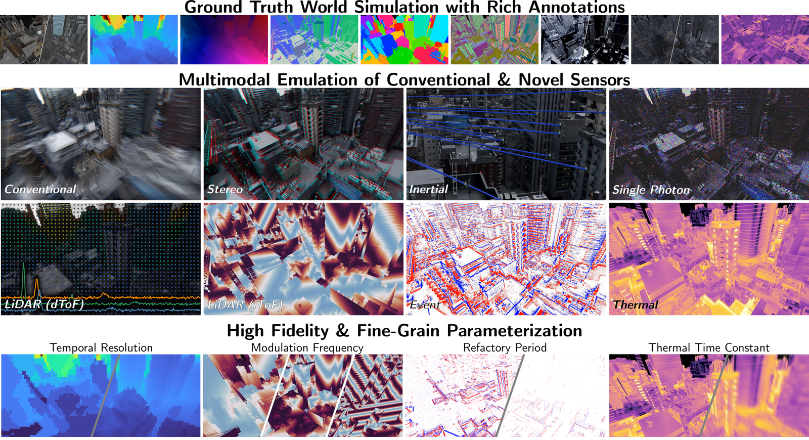
The one architectural decision that matters is the split between two layers.
The world simulation layer is Blender. It renders the clean scene plus
ground truth: depth, normals, optical and scene flow, segmentation, point maps,
direct and indirect diffuse and specular passes, poses, intrinsics, and a
temperature field from a heat solver (more on that below). It is a big piece of
Python: the package is about 19,800 lines, and visionsim/simulate/blender.py
alone is 3,746 of them (reasoned, wc -l).
The sensor emulation layer takes those clean frames and turns them into what a particular device would have recorded. Because the layers are separate, one render can be replayed through any number of sensors, and a parameter can be swept "at zero extra rendering cost", in the paper's words.
The hard part is the frame rate. An event camera or a single-photon camera lives at thousands to hundreds of thousands of frames per second; rendering that many path-traced frames is not feasible. VisionSIM's answer has three parts: render on a pool of machines over RPC, remap animation keyframes so a physics simulation can be sampled at any rate, and render only at the scene's native rate and fill the gaps with a learned video interpolator, RIFE. The released dataset shows the ratios (reported): 100 indoor scenes, each a 24-second trajectory rendered at 100 fps, 1000 x 1000, as a stereo pair, for 480,000 ground-truth views. From those it emulates a single-photon camera at 16 kHz (160x interpolation), an event camera at 4 kHz (40x), a 25 fps conventional camera, both LiDARs, thermal, and an IMU at 250 Hz. The project page says the dataset is "coming soon", with a prerelease available.
That interpolation step is the price of the design. A 160x interpolated frame is a guess between two real ones, and the single-photon and event models are only as good as those guesses. The paper says the render-then-interpolate path preserves "high fidelity to fully rendered sequences"; I did not test that.
Event cameras: change, not frames
An event camera has no frames. Each pixel remembers a log brightness level and
fires an ON or OFF event whenever the current log brightness moves more than a
threshold away from it, then resets its memory. VisionSIM's model is a port of
v2e, and reading
visionsim/emulate/dvs/v2e/emulator.py gives the full chain:
- Map intensity (0 to 255) through
lin_log: linear below 20, natural log above. - Low-pass it with a first-order filter whose time constant shrinks with brightness. This is the photoreceptor bandwidth: dim pixels respond slowly.
- Give every pixel its own ON and OFF threshold, drawn once from N(0.2, 0.03) and clipped at 0.01. Real sensors have this mismatch.
- Count crossings with a floor division of the log change by the threshold, spread them evenly through the frame interval, and drop any that fall inside a pixel's refractory period.
- Add leak events (slow drift of the memory) and shot-noise events.
The paper's headline failure mode for events is "refractory drop-out". The project page shows the other one: when a lamp switches on, every pixel changes at once and the array floods. I ran both through my port, with leak and shot noise off so the counts are the model's own.
The threshold sweep is what you would expect (measured): a disc crossing a 96 x 96 checkerboard for half a second gives 26,377 events at threshold 0.1, 10,916 at the default 0.2 and 4,379 at 0.4. Roughly inverse in the threshold, steeper at the low end where noise-free texture starts to count.
The lamp is the interesting one (measured). Stepping the board from a quarter to four times its brightness, four stops, fires 131,917 events across its 9,216 pixels, about 14 per pixel, because ln 16 is 2.77 log units and the threshold is 0.2. Two things decide when they arrive:
- The photoreceptor cutoff. The
EventEmulatorclass defaults to 30 Hz; thevisionsim emulate.eventsCLI defaults to 200 Hz. Same events, very different timing: with 200 Hz, 95% of the burst lands in the first millisecond; with 30 Hz it takes about 30 ms to reach 99%. A user who calls the class directly gets a different sensor from a user of the CLI, and neither default is wrong, but it is worth knowing which one you have. - The refractory period. In this implementation a suppressed crossing is not deleted. The pixel's memory is only updated by the events that actually fired, so the unfired change is still there next frame and fires then. The total stays at 131,917 for 0.5 ms and 2 ms; only the timing stretches, to about 20 and 40 ms. At 10 ms, each pixel emits one event per 10 ms and 1,806 events are still queued 200 ms after the switch. Whether that matches a real pixel is a question for a datasheet; it means "drop-out" here is really delay, unless the change reverses before the backlog drains.
Reported: event counts emulated from RGB video of an auditorium differ from a real Prophesee EVK4 recording by 1.5% for ON events and 5.8% for OFF. The paper is candid that the bandwidth and refractory period used the generic DVS model, not the EVK4's.
Single-photon cameras: one bit per pixel
A SPAD pixel either sees a photon in its exposure or it does not. Photon
arrivals are Poisson; the pixel can count at most one, so the frame is a
Bernoulli draw with probability , where is the flux
and the exposure. VisionSIM's emulate_spc is that, literally one line:
rng.binomial(1, 1.0 - np.exp(-img * factor)). The inverse, spc_avg_to_rgb,
averages many binary frames and takes . The factor maps
the renderer's linear intensity to photons and absorbs dark counts and fill
factor; there is no absolute radiometry in a Blender scene, so someone has to
pick it.
What the inversion costs (measured, 2,000 pixels per flux level, median relative error): one frame is useless, as the project page says ("on its own, looks like noise"). At a flux of one photon per frame, 64 frames give 11.4%, 512 give 4.0%, 4,096 give 1.4%. The dark end needs frames just to see a photon: at 0.01, even 512 frames leave 37.7% error. The bright end saturates: at 8 photons per frame, the detection probability is 0.9997, and 84% of pixels fired in all 512 frames, which inverts to the clamp rather than the flux. That saturation is why the project page's lamp scene says summing eight frames "lets the room emerge" but needs more frames and the inverse response to see both the table and the lampshade.
The storage side is a small, good idea (reported): binary frames are kept as one big bit-packed NumPy array, eight pixels per byte, memory-mapped, so a training loop can pull single pixels from millions of frames without decoding an image codec. On the hardware side, the emulated Pi-Imaging SPAD statistic reached 0.221 against a measured 0.229; the paper blames the source camera's unknown white balance and response, not the sensor model.
Indirect time-of-flight: depth from phase
An iToF camera modulates its light and correlates the return against shifted copies of the code; each correlation is a "tap". With a sinusoid, the taps sample a cosine, and the phase of that cosine is the round-trip delay. Depth is , and since phase lives on a circle, anything past the unambiguous range folds back.
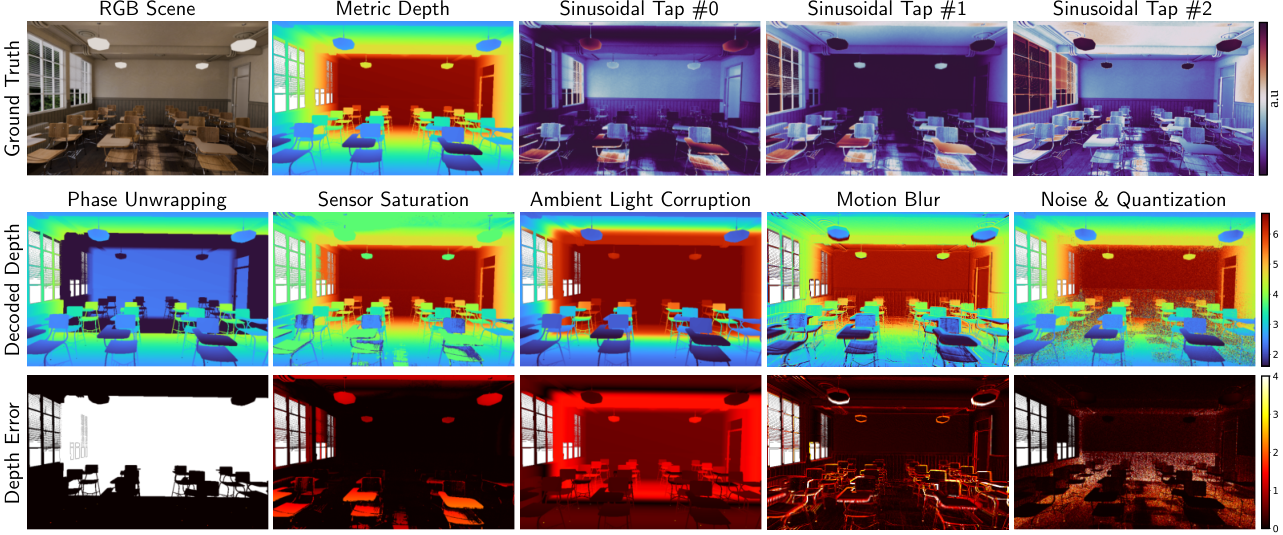
The paper's first failure case uses 35 MHz, "yielding an unambiguous depth of
only ~4.3 meters". The arithmetic agrees: 299,792,458 / (2 x 35 MHz) is
4.28 m (reasoned), and my port of the 3-tap deltaSin pipeline decodes a
surface at 4.5 m as 0.217 m (measured), exactly 4.5 minus 4.28.
Then the code. visionsim/emulate/itof/ is careful about codes: it ships
conventional and delta sinusoids, square waves, single and double ramps,
multi-frequency sinusoids and Hilbert codes, with a decoder for each. But
simulate_measurements returns exactly
(exposure / period) * (beta * correlation + ambient * kappa * albedo) and
nothing else (reasoned, from the source). No shot noise, no read noise, no
full-well clipping, no ADC, no tap motion; the CLI's emulate.itof adds none
either. Four of the five failure modes in Figure 2 (saturation at 50k
electrons, the ambient corruption, the 100 ms motion artefact, read noise of
10 electrons with a 12-bit ADC) are not in the package I installed.
That has a measurable consequence. Ambient light adds the same constant to
every tap, and the sinusoid decoder fits [1, cos, sin] by least squares, so
the constant goes into the first coefficient and the phase does not move. In my
port, decoded depths with ambient equal to the laser's power are identical to
those with none, at every depth (measured). Ambient only hurts through the
shot noise it brings, so I added Poisson noise myself: at 20 MHz, with ambient
at a fifth of the laser power, RMS error at 4 m goes from 20.7 cm to 39.2 cm,
and at 6 m from 29.7 cm to 133 cm (measured, my noise model, not theirs).
If you want Figure 2's ambient row from the released package, you will need to
add the noise yourself.
One number in the paper I cannot reconcile. Against a real Chronoptics iToF camera, the emulator's mean phase error is 0.13 rad, which "at a 40 MHz modulation frequency, translates to a mean depth error of about 5.3 cm" (reported). By the same the decoder uses, 0.13 rad at 40 MHz is 7.75 cm (reasoned). Either the phase or the depth is off, or a factor I do not see is in play.
Direct time-of-flight: pileup and glare
The single-photon LiDAR model in the paper is the most complete forward model in it (reported): per-pixel field-of-view masks that integrate albedo over depth squared into a transient histogram, convolution with the instrument response, a constant ambient rate filtered to the laser band, Poisson arrivals, and a non-paralyzable dead time that produces pileup. Pileup is the effect where a bright early return blinds the detector for the rest of the cycle, so the histogram skews early and the object reads closer than it is. That "range walk", plus glare ghosts from a retroreflective sign, is what the digital-twin case study reproduces on an Adaps ADS6311, lowering RMSE by about 1.53 m once the impulse response, pileup and glare are modelled. The model is written in PyTorch and differentiable, which is how the impulse response was fitted from real captures.
None of it is in the visionsim package I read (reasoned). The two dToF
examples, examples/sensors/ewh_spc.py and edh_spc.py, import a separate
SPCSim library and load renders from a hard-coded path under one author's
home directory. The paper mentions a unit-aware configuration system built on
pint and ruamel.yaml; neither is a dependency. The dToF results may well be
reproducible with SPCSim; they are not reproducible with pip install visionsim alone. For what a real 1535 nm LiDAR adds on top, see
Hesai Kosmo.
Thermal: heat first, then light
This is the part I would point a colleague at. Most simulators fake thermal by painting a temperature texture on each object. VisionSIM computes the temperature (reported, and read in code):
- Light becomes heat. For an opaque Lambertian surface, whatever is not reflected is absorbed: . The irradiance comes straight from the renderer's diffuse passes, baked to a texture per timestep and resampled to mesh vertices. Turn a lamp off in Blender and its heat goes too; nobody authors a thermal boundary condition by hand.
- Heat spreads. A finite-element heat equation on the mesh, with
convection and linearised radiation to ambient folded into one constant
stiffness matrix, so it is assembled once and only the right-hand side
changes per frame. Real asset meshes are full of slivers and non-manifold
junk; the Laplacian is an intrinsically mollified cotangent operator
(
robust-laplacianis a dependency) so it stays well conditioned without remeshing. Hot tea is a Dirichlet condition on the tagged inner surface. - Heat becomes LWIR radiance. A graybody shader writes : emission scaled by emissivity plus the reflection of the surroundings. That second term is why polished metal "looks cold" in a thermal image.
The visionsim/simulate/heatsim/ package is about 5,900 lines (reasoned)
and runs inside Blender; the quick-start example is a 600-second heat solve on
the Ultramodern scene at a 1 s timestep.
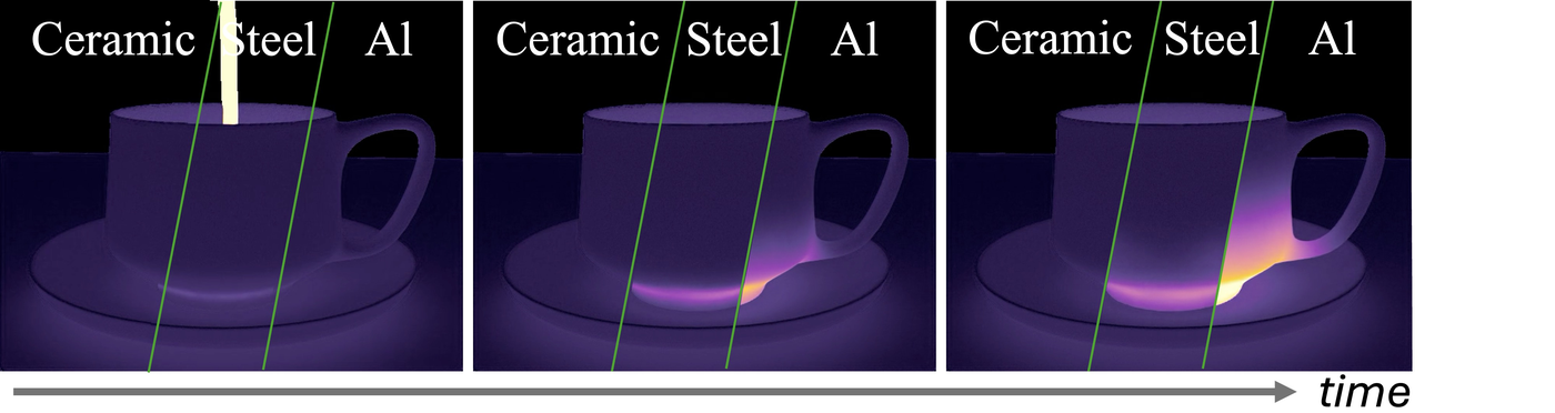
The diffusivity numbers explain the figure on their own. The time for heat to cross a wall of thickness scales as . For a 3 mm wall that is about 4.5 s for ceramic, 0.48 s for steel and 0.09 s for aluminium (reasoned, a scaling estimate, not their solver). So in a four-second clip the aluminium is through, the steel is through, and the ceramic has barely started, which is what the figure shows.
The last stage is the camera itself. A microbolometer pixel is a membrane with
heat capacity, so its reading lags the scene: ,
with of 5 to 15 ms for commercial uncooled detectors. Discretised with a
zero-order hold it becomes one line, with
. At 60 fps and 10 ms the paper gives
and says a hot pixel reaches about 90% "in about three frames". The arithmetic
gives 81% after one frame and 96% after two (reasoned), so three frames is
generous. More important: I searched the repository for the filter and did not
find it (reasoned, grep for bolometer, time constant and the IIR form
across visionsim/). The heat solver and the graybody render are there; the
sensor lag that the paper's Figure 1 sweeps as "thermal time constant" is not,
at this commit.
Does it match real sensors?
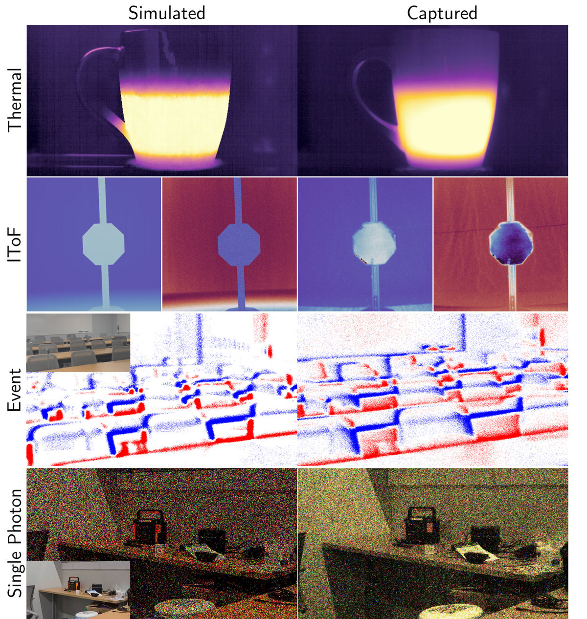
The paper's sim-to-real section (reported, all of it):
| sensor | real device | agreement |
|---|---|---|
| thermal | FLIR Boson | heating curve within 7.6% MAE of the mug's dynamic range, 4 s |
| iToF | Chronoptics | 0.13 rad mean phase error |
| events | Prophesee EVK4 | counts within 1.5% (ON) and 5.8% (OFF) |
| single-photon | Pi-Imaging SPAD | 0.221 vs 0.229 |
| dToF | Adaps ADS6311 | RMSE lowered by about 1.53 m with IRF, pileup and glare |
Each is one scene. The authors say so in their limitations: one commercial LiDAR, a small set of scenes, and every evaluation open-loop. The sensor-suite case study (RGB plus events against single-photon plus IMU, judged by a zero-shot detector reaching 90% confidence on the second) measures the whole reconstruction-plus-detector pipeline, not the sensors, and the paper says that too.
What I would use it for, and what it costs
What it gets right. The two-layer split is the correct design, and the code
is serious about it: one render, then sweep event thresholds, iToF codes or
SPAD exposure without touching Blender. The passive SPAD and event emulators
also run on any video you already have; the paper's dataset-migration examples
emulate single-photon frames from XVFI and events from a Genesis render. That
part needs no Blender at all: visionsim emulate.events and visionsim emulate.spad take a folder of frames.
What I would check first.
- Which event-camera cutoff you are getting: 30 Hz from the class, 200 Hz from the CLI.
- That refractory suppression delays rather than drops, in case your downstream code assumes the opposite.
- That
emulate.itofis the ideal correlation model. Add shot and read noise and a full-well clip before trusting it in daylight. - That dToF needs SPCSim and the bolometer lag needs writing, for now.
What it costs. Blender 3.6 or newer on PATH for any rendering, a GPU for
the thermal solver to be pleasant, and a render farm if you want the dataset's
100 fps at 1000 x 1000. I rate runsOn as a workstation. The licence is
GPL-3.0-or-later, with a commercial licence on request; contributions come in
under MIT. If you are building a product on it, that GPL matters more than any
number above.
If you have used Blender as a scene generator or a real multi-sensor rig, the appeal is obvious: synchronisation and calibration are free when the sensors are equations. The catch is the same one every simulator has. The equations are only as honest as their parameters, and the most interesting ones here are still in the paper rather than the package.