2026-11-12 · 23 min · small-models · on-device · distillation · mixture-of-experts · pruning · linear-attention · gguf · benchmarks
A 3:51 narrated explainer, drawn in code. Every number and picture in it is this article's own; the sources are below.
› transcript
Here is a small language model with three point one billion parameters. On a phone, only about half of them need the fast memory. Where does the other half go? Hi, I'm Basalt! Today we open up Raon one nano, from KRAFTON, and count where every parameter lives. Chapter one. Half is a lookup table. A normal model turns each token into one vector at the bottom of the stack, and that is the last time it consults the vocabulary. Raon also keeps a second table, with one long row per token. The row is cut into twenty-four slices, one for each layer. Each layer, after its attention and its feed-forward block, reads its own slice back in, through a gate that the hidden state controls. The table holds one point six billion parameters. But a forward pass only ever fetches one row. It never multiplies by the rest. Follow a single token through it. The id selects one row of six thousand one hundred and forty-four numbers. At four bits, that is about three and a half kilobytes. Each of the twenty-four layers takes its two hundred and fifty-six numbers, and multiplies them by a gate computed from the hidden state. The result is projected back to full width and added to all four residual streams. Chapter two. Where the bytes live. At four bits, the weights every token multiplies come to about point eight six gigabytes. The table is another point nine, and it can stay in host memory or on flash. The reference PyTorch code expands its six attention caches to thirty-two full heads. That is about eighteen times too much for a phone. Keep only the latent, and it is six thousand nine hundred and twelve bytes per token. The other eighteen layers keep a fixed state that never grows. Chapter three. From experts to dense. Take one mixture of experts layer from Qwen three, with a hundred and twenty-eight experts and eight active per token. Score every expert on calibration text. Keep eight. The best score multiplies importance by diversity, so the chosen experts do different work instead of repeating each other. Stack the eight side by side, and they become one dense feed-forward block, six thousand one hundred and forty-four wide. Then distil from the original mixture of experts, matching its output distribution. The paper draws it like this. Experts are scored and chosen. Then concatenated, and distilled with a K L loss from teacher to student. The paper's own result. After about four billion tokens, the diverse pick averages fifty-eight point one percent. Pruning a dense teacher of the same total size gets fifty-one point eight four. But Raon one nano is not that recipe, applied as written. Compare the two models side by side. Its width is one thousand five hundred and thirty-six, not the teacher's two thousand five hundred and sixty. It has a per-layer table that the teacher never had. And it trained on three trillion more tokens. The paper never tests whether its head start survives that. Parameters you look up are cheaper than parameters you multiply. Nano puts half its weights where only one row per token is ever read. To recap. Half the model is a lookup table. Only the weights that multiply need fast memory. And a diverse pick of experts is a better start than a pruned dense model. Every source is in the full article. I'm Basalt. Bye!
Why read this
Solidtop 85%Counts Raon-1 nano's 3.1B from the headers, shows which 1.6B can leave the accelerator, and checks the MoE-to-dense paper against nano's own configs.
- Original analysis
- Runs on a laptop CPU
- Concrete numbers to act on
LLM architectureApache-2.0Practitioner model
How this was scored
- Is it new?
- 1 of 3: An incremental tweak
- Can I trust it?
- 2 of 3: Measures key facts from files, code or configs
- Can I run it?
- 2 of 3: Open code or weights with real limits
- Will I understand it?
- 2 of 3: Mechanism from first principles with figures
- Can I act on it?
- 2 of 3: A concrete recipe, numbers or comparison
- Will it last?
- 1 of 3: Relevant for months
- Does it affect many?
- 1 of 3: A specialist community
- Only here?
- 2 of 3: A teardown or measurement few others did
Score 59 of 100, ranked 478 of 740 rated articles. Each question is answered 0–3 by hand, and a 3 is rare. How articles are scored
On 2026-11-11 KRAFTON AI posted: "We're releasing Raon-1 nano, an effective 1.5B dense LLM with per-layer embeddings and 3.1B total parameters." The rest of the post gives the lineage in one sentence: "We pruned and distilled Raon-1 mini preview (30B-A4B) using our MoE-to-Dense approach, then further trained it on 3T tokens, followed by SFT, OPD, and RL." The weights are on Hugging Face under Apache 2.0 at KRAFTON/Raon-1-nano, and the method has its own paper, Pruning and Distilling Mixture-of-Experts into Dense Language Models, accepted as a NeurIPS 2026 oral.
Two phrases in that post carry the whole design: "effective 1.5B" and "MoE-to-Dense". The first is a statement about
memory placement, the second about where the starting weights came from. I did not download the model. I range-read the
headers of the two safetensors shards, the tied LM-head file, the MTP file and KRAFTON's own Q4_K_M GGUF, read
modeling_raon1_nano.py and the paper, and compared the configs of nano and its teacher. Nothing below was run on a device.
- architecture
- Raon1NanoForCausalLM
- task
- text-generation
- library
- transformers
- license
- apache-2.0
- safetensors
- 4 shards
- largest file
- 3.19 GB
- files
- 23
- downloads
- 446
- likes
- 64
The Hub counts 3.53B because it adds model-tied-lm-head.safetensors, a second copy of the 399M tied embedding. The main model is 3,130,797,328 parameters.
repo last modified 2026-11-11
Half the checkpoint is a lookup table
Start with the count. Summing every tensor shape in model-00001-of-00002.safetensors and model-00002-of-00002.safetensors:
| Part | Parameters |
|---|---|
Per-layer embedding table, per_layer_inputs.table, 259,840 x 6,144 | 1,596,456,960 |
Token embedding, embed_tokens (tied to the LM head) | 399,114,240 |
| 24 decoder layers: attention, MLP, Raon-mHC mixers, per-layer gates, norms | 1,125,787,152 |
| Per-layer input projection and its norm | 9,437,440 |
| Final norm | 1,536 |
| Main model | 3,130,797,328 |
MTP module (mtp/model.safetensors, one extra layer) | 54,841,898 |
The second shard holds exactly one tensor, the per-layer table. Take it away and 1,534,340,368 parameters remain. So both numbers in the post are right: 3.1B in total and 1.5B "effective", where effective means everything except the table. It still includes the 399M token embedding, which in this model is not free, because the LM head is tied to it and every generated token multiplies the hidden state by all 259,840 rows. Strip that too and the transformer body is 1.14B.
Hugging Face's badge on the repo says 3.53B. That figure adds model-tied-lm-head.safetensors, a second copy of the
embedding for runtimes that want an explicit lm_head. I hashed three 4 MB windows (start, middle, end) of both tensors
and they matched byte for byte, so the badge double-counts 399M parameters. It also misses 192 parameters: the 192
scalar tensors (shape [], eight per layer) that the Hub's counter skips.
What a per-layer embedding is
An ordinary decoder looks up one vector per token at the bottom of the stack and never consults the vocabulary again until
the output head. A per-layer embedding (PLE) gives every token a second, private vector for each layer. Gemma 3n
introduced the idea for phones, and Gemma 4's E2B and E4B use it; this site's Gemma 4 article and
the Nemotron 3.5 Bolt teardown cover Google's version. Raon's version, read from
Raon1NanoPerLayerInputs and Raon1NanoPerLayerInputGate, has two halves.
At the bottom of the model, for token with main embedding , it builds 24 vectors of width 256, one per layer :
is the 259,840 x 6,144 table: each row is a token, cut into 24 slices of 256. is a 6,144 x 1,536 projection of the ordinary embedding, so a token's per-layer input is half "what this token means in general" and half "what this token means to this layer specifically".
Then, inside layer , after the attention and the MLP have run, the layer reads its slice back in:
is the mean of the four residual streams (Raon uses four parallel streams, more on that below). The gate is 1,536 to 256, the projection 256 to 1,536, and the result is added to every stream. The current hidden state decides how much of the token's per-layer vector gets in; the vector itself is fixed per token.
The property that matters for a device is in the first equation. is an index, not a matrix product. A forward pass needs one 6,144-wide row per token and never touches the other 259,839. Everything else in the model is a weight that every token multiplies by. That is the line between "effective" and "total", and why KRAFTON can count 1.6B parameters as not running.
Where the bytes have to live
A weight that every token multiplies has to be read in full for every token, so it belongs in the fastest memory you have: the GPU's VRAM, an NPU's SRAM and DRAM budget, a phone's share of unified memory. A table read one row at a time can sit in host RAM or be memory-mapped from flash, because a row at 4 bits is only 3,456 bytes.
KRAFTON's llama.cpp branch (raon-1-nano-preview in krafton-ai/llama.cpp)
reuses Gemma 3n's tensor name for the table, per_layer_token_embd. In that fork's src/llama-arch.cpp the name is registered
as LLM_TENSOR_LAYER_INPUT with op GGML_OP_GET_ROWS, and src/llama-model.cpp assigns input tensors to
dev_input = { cpu_dev, … }. I read the tensor table and the device assignment, not nano's graph code, so the safe
reading is: per the fork's tensor table, the table loads to the CPU side even with every layer offloaded.
The calculator below adds it up. Pick the precision, move the table on or off the accelerator, and slide the context.
Some anchors from it. At 4-bit, the compute weights take about 0.86 GB and the table another 0.90 GB. Keeping the table in host memory nearly halves the accelerator's weight budget, which is the whole point of the architecture. At BF16 the split is 3.07 GB against 3.19 GB.
KRAFTON's own raon-1-nano-Q4_K_M.gguf is 2,082,677,632 bytes. Parsing its header with a 25 MB range request:
per_layer_token_embd is stored at Q4_K and takes 898.0 MB, 43% of the file. token_embd is Q6_K at 327.4 MB. The
remaining 845 MB are the 24 blocks, mixed Q4_K, Q6_K and Q8_0, plus a few F16 and F32 tensors. That is a different
choice from NVIDIA's Gemma-based Bolt, whose GGUF kept its table at Q8_0, and the same floor as Qwen3.8-Flash-Next,
whose quantizers would not take its tables below 4-bit. A table that only lives in host RAM costs little to keep at higher
precision, so storing it at Q4_K is a bet on phones, where host RAM and accelerator memory are the same pool.
The cache is small if the runtime keeps it small
18 of nano's 24 layers are Raon Delta Attention (RDA), a gated delta-rule linear attention. Each keeps a fixed state of 16 heads x 128 x 128 in FP32, 1 MiB per layer, and a three-token convolution window, for about 19.5 MB in total at any context length. Only six layers (the fourth, eighth, and so on) are multi-head latent attention, MLA, with a KV cache that grows.
The card says that cache is "about 7 KiB per token in BF16". That checks out for a latent cache: MLA compresses keys and values into a 512-wide latent, plus 64 key channels shared across heads, so six layers at 576 values and 2 bytes each come to 6,912 bytes per token. At the full 262,144-token context that is 1.81 GB, and at 32K it is 226 MB.
The reference PyTorch code does not store the latent. Raon1NanoMLA.forward expands it to 32 heads of 192-wide keys and
128-wide values before cache.update, which is 122,880 bytes per token (),
about 18 times as much. That is fine for a correctness reference and wrong for a phone. The GGUF header declares a key length of 576 and a value length of 512 for the MLA layers, which suggests the llama.cpp
branch caches the latent, possibly with the value as a view of the key; I did not trace its cache code. The calculator's
4-bit setting also assumes 4.5 bits everywhere, while the shipped Q4_K_M keeps more precision: its embedding and blocks
together take about 1.17 GB (327.4 MB plus 845 MB).
The other 1.5B: a hybrid built to forget
The body is as unusual as the table. From config.json and the card:
- Raon Delta Attention in 18 layers. A delta rule updates a matrix state by writing the error between the value and what the state
already predicts for the key. RDA, per the Raon-1 mini card, "decouples the erase and write gates of Kimi Delta Attention":
torch_recurrent_rdadecays the state, computeserror = v - S k, and writes it with strength , while a separate write gate rescales the value. The decay is bounded below by in log space. - Gated MLA in six layers, with no positional encoding at all (NoPE). The 64 "rope" channels in the latent are never rotated; they are just extra key channels shared across heads. Order comes from the RDA layers' recurrence.
- Raon-mHC with four residual streams instead of one, KRAFTON's cheaper version of DeepSeek's manifold-constrained hyper-connections. It costs 5,014,512 parameters in all.
- SwiGLU MLP of width 6,144, the largest single block: 679M of the 1.13B in the layers.
The card warns that the PyTorch implementation "processes prompt tokens sequentially, so long-prompt prefill can be slow".
torch_recurrent_rda is a Python loop over tokens. Use the vLLM or llama.cpp branches, which have fused kernels.
Turning a mixture of experts into one dense FFN
The paper behind "MoE-to-Dense", by Junhyuck Kim and five co-authors at KRAFTON and KAIST, starts from a deployment complaint: an MoE needs every expert in memory even though each token uses a few, and pruning experts still leaves an MoE. Their target is a plain dense transformer whose size equals the teacher's active parameters.
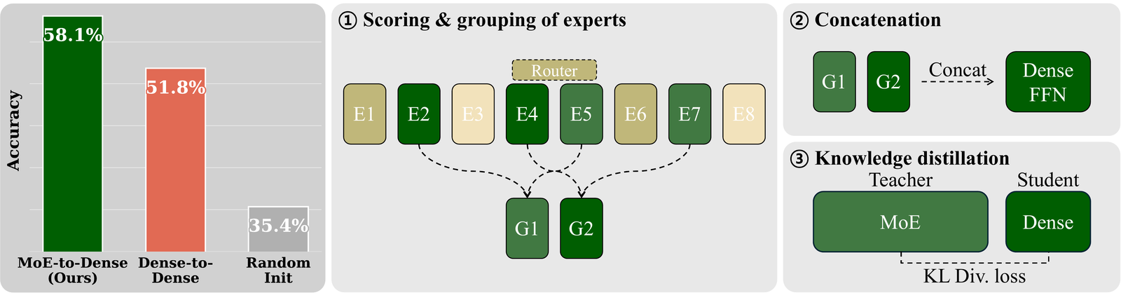
Take one MoE layer with experts, top- routing and SwiGLU experts of width . The construction:
- Score every expert on a calibration set (512 WikiText-103 sequences of 2,048 tokens).
- Select the top experts.
- Group them into groups and average weights within each group, weighted by score. With each group is one expert and nothing is averaged.
- Concatenate the groups' gate and up projections row-wise and down projections column-wise. The dense FFN has width , and because the intermediate activations of each block are untouched, the dense layer computes exactly the sum of its blocks.
- Scale each block's down-projection by a fixed (uniform , or by score), because no router is left to weight them per token.
- Distil from the MoE teacher with forward KL on the logits.
For Qwen3-30B-A3B (, , ) that gives a 6,144-wide FFN and a 3.3B dense student. Attention, embeddings and norms are copied across unchanged.
The interesting choice is step 1. Earlier merging work (MC-SMoE, HC-SMoE, MergeMoE) scores experts by how often the router picks them. Frequent experts are generalists, and generalists overlap. The paper's best score, DO-ACP, combines a REAP-style importance (conditional routing probability times output norm) with a D-optimal set objective over the experts' output Gram matrix :
A determinant is a volume. Two experts whose outputs point the same way span almost no extra volume, so the second one adds almost nothing to however important it is alone. The objective is monotone submodular, so greedy selection gets within of the optimum, and the paper does it with Schur complements in .
The widget runs that greedy rule on twelve invented experts, four of them near-twin generalists. Slide and compare what plain top-K by importance keeps with what the log-det objective keeps.
With four slots, top-K spends all four on the twins. The log-det rule takes the best twin and then three experts that do different work. On Qwen3-30B-A3B the paper measures the same effect: D-optimal selection raises the effective rank of the eight chosen experts from 6.07 to 7.37 over conditional probability alone, and from 6.31 to 6.93 over ACP.
What the paper's numbers show
The sweep covers 7 scoring methods, 5 grouping methods, 2 down-projection scalings and : 350 configurations ranked by perplexity, then the best for each of the 35 scoring and grouping pairs distilled for 0.3B tokens.
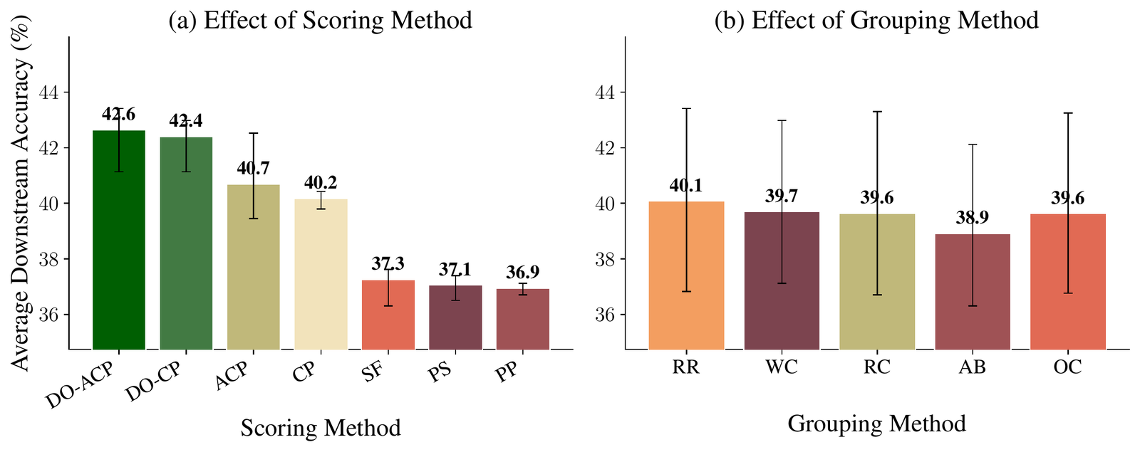
- Every one of the top seven configurations uses : pure pruning, no weight averaging. Merging gives a lower perplexity before distillation and a worse model after it.
- At 0.3B tokens, DO-ACP reaches 43.41% average accuracy over Winogrande, HellaSwag, ARC-Easy, ARC-Challenge and MMLU. MC-SMoE's metrics in the same framework give 36.31%, HC-SMoE's 37.52%, Minitron-style pruning of a dense Qwen3-32B to 3.4B gives 33.28%, and random initialisation 30.15%. The teacher scores 79.65%.
- Forward KL wins. Reverse KL costs 6.24 points, and adding hidden-state MSE costs 1.91.
- Over about 4B tokens the order holds: DO-ACP 58.10%, frequency scoring 53.46%, dense-to-dense 51.84%, a random FFN under the teacher's attention 45.44%.
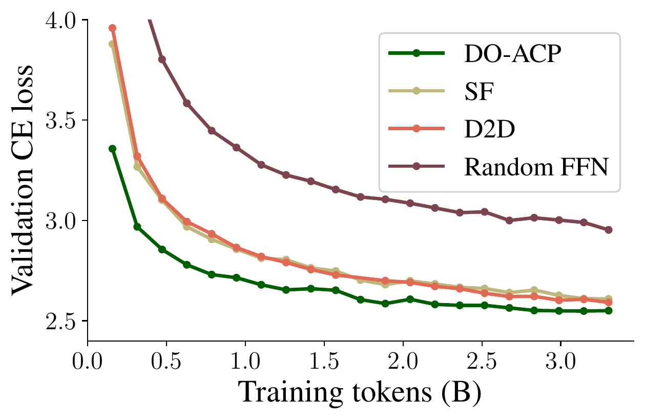
The cost argument is clean too. The MoE teacher activates 3B parameters per token while the dense Qwen3-32B teacher runs all 32B, so a distillation step took 73 s against 116 s on two B200s, 1.6 times faster.
The paper is just as clear about where it stops. After 4B tokens its 3.3B student still trails a pretrained Qwen3-1.7B, 58.10% against 66.63%. The method is an initialisation that saves training, not a substitute for training.
Nano is not that recipe, applied
This is where the release and the paper part ways, and the configs make it plain. The paper's construction keeps the
teacher's hidden width, its attention and its embeddings, and sets the FFN to . Here are Raon-1 mini
preview's config.json and nano's side by side:
| Raon-1 mini preview | Raon-1 nano | |
|---|---|---|
| Hidden size | 2,560 | 1,536 |
| Layers (RDA + MLA) | 25 (18 + 7) | 24 (18 + 6) |
| RDA heads / MLA heads | 40 / 40 | 16 / 32 |
| Query LoRA rank | 576 | 512 |
| FFN | 128 experts of 1,088; 6 routed + 1 shared | dense, 6,144 |
| Activation | SiTU-GLU | SwiGLU |
| LM head | untied | tied |
| Per-layer embedding | none | 24 x 256 |
| Tokenizer | tokenizer.json, sha256 47752d33… | identical file |
A literal application would give a 2,560-wide, 25-layer model with an FFN of 6 x 1,088 = 6,528 or, counting the shared expert, 7,616, and an untied head. Nano is narrower, one layer shorter, has fewer heads, a different activation, a tied head, and 1.6B parameters of per-layer table that the teacher never had. 6,144 is not a whole number of mini's experts. So getting from the MoE to nano took some reduction of width, depth and heads that the paper does not describe, plus a component the teacher does not have. How it was done is not published. The card's phrase "MoE-to-Dense pruning and knowledge distillation" covers all of that, and none of it is described. The paper itself never mentions Raon; its experiments are on Qwen3, DeepSeek-V2-Lite and GPT-OSS.
What survives the comparison: the tokenizer files are byte-identical, so mini's logits can teach nano directly, which both logit distillation and on-policy distillation from mini (the "OPD" in the post) need. The site's Inkling-Small article goes through what on-policy distillation buys a small reasoning model.
The other thing to keep in mind is scale. The paper's evidence is at 0.3B and 4B tokens. Nano was then trained on 3T tokens, 750 times the paper's longest run. Whether a better initialisation still shows after that much training is exactly what the paper does not test. I would expect most of the advantage to wash out, and some to remain in the compute KRAFTON saved getting started.
Reading the benchmark table
The README's table compares nano against Qwen3.5 2B, Gemma 4 E2B, MiniCPM5 2B and LFM3 1.7B on 15 rows. The repo also ships it as an image, and the two disagree.
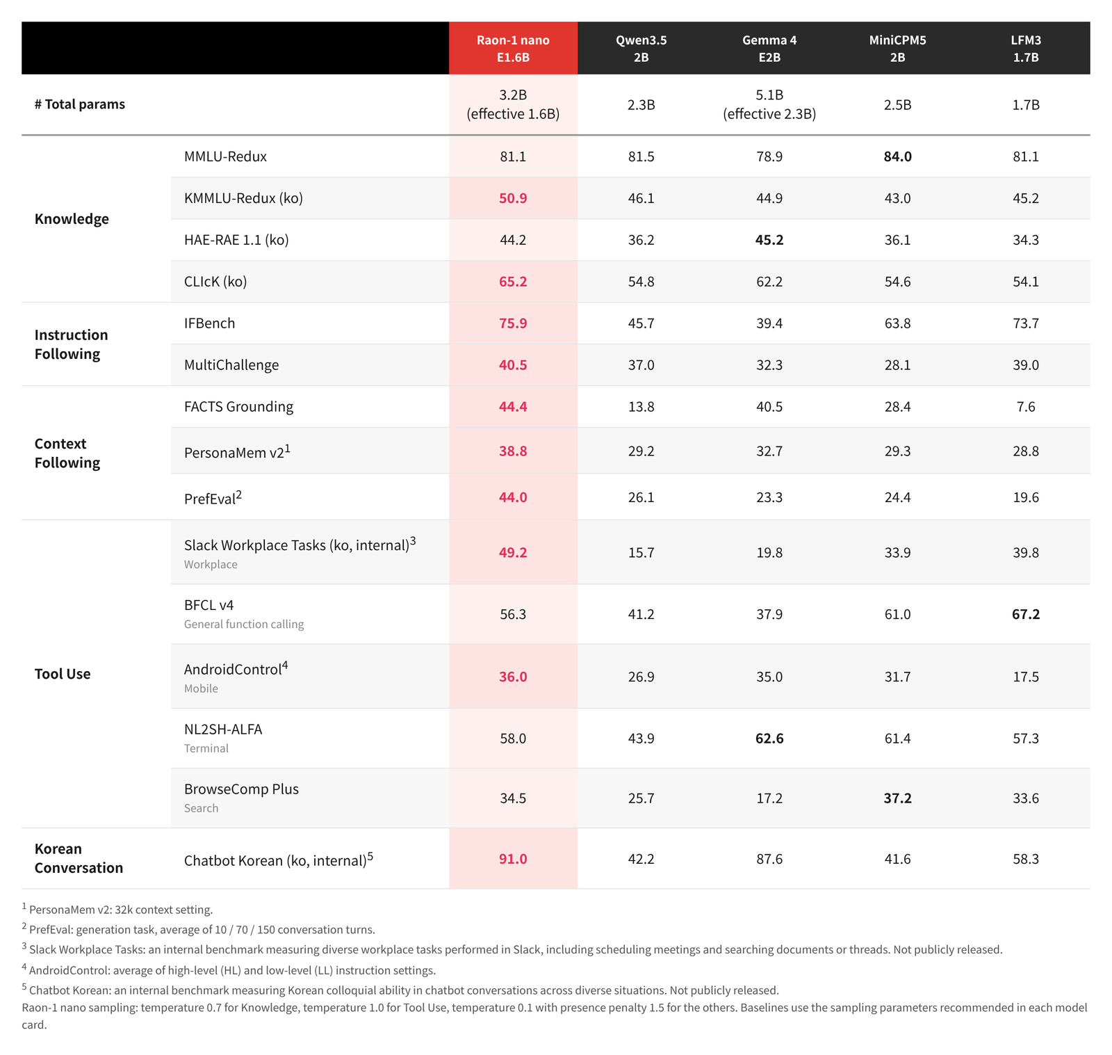
The parameter mismatch reconciles if the image counts the MTP module: 3,130,797,328 plus 54,841,898 is 3.19B, and
1,534,340,368 plus 54,841,898 is 1.59B. The card says the MTP module is not used by normal from_pretrained() or
generate() calls, so the README's 1.5B and 3.1B are the right numbers for the model you run.
On the scores themselves, nano leads 10 of the 15 rows. Where it does not: MMLU-Redux (81.1 against MiniCPM5's 84.0), HAE-RAE (44.2 against Gemma's 45.2), BFCL v4 (56.3 against LFM3's 67.2), NL2SH-ALFA (58.0 against Gemma's 62.6) and BrowseComp Plus (34.5 against MiniCPM5's 37.2). The widest public lead is PrefEval, 44.0 against 26.1, followed by PersonaMem at 38.8 against 32.7; on IFBench (75.9 against 73.7) and FACTS Grounding (44.4 against 40.5) the margins are a few points. Two of the strongest rows, Office Work Bench at 49.2 and Chatbot Korean at 91.0, are internal and "Not publicly released", so nobody outside KRAFTON can check them. For a tool-use model the public tool rows matter most, and there nano is third of five on BFCL v4 and on NL2SH-ALFA, second on BrowseComp Plus, and first only on AndroidControl, by one point.
The X post carried its own chart, and it is drawn differently from the one in the repo.
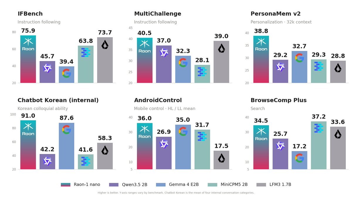
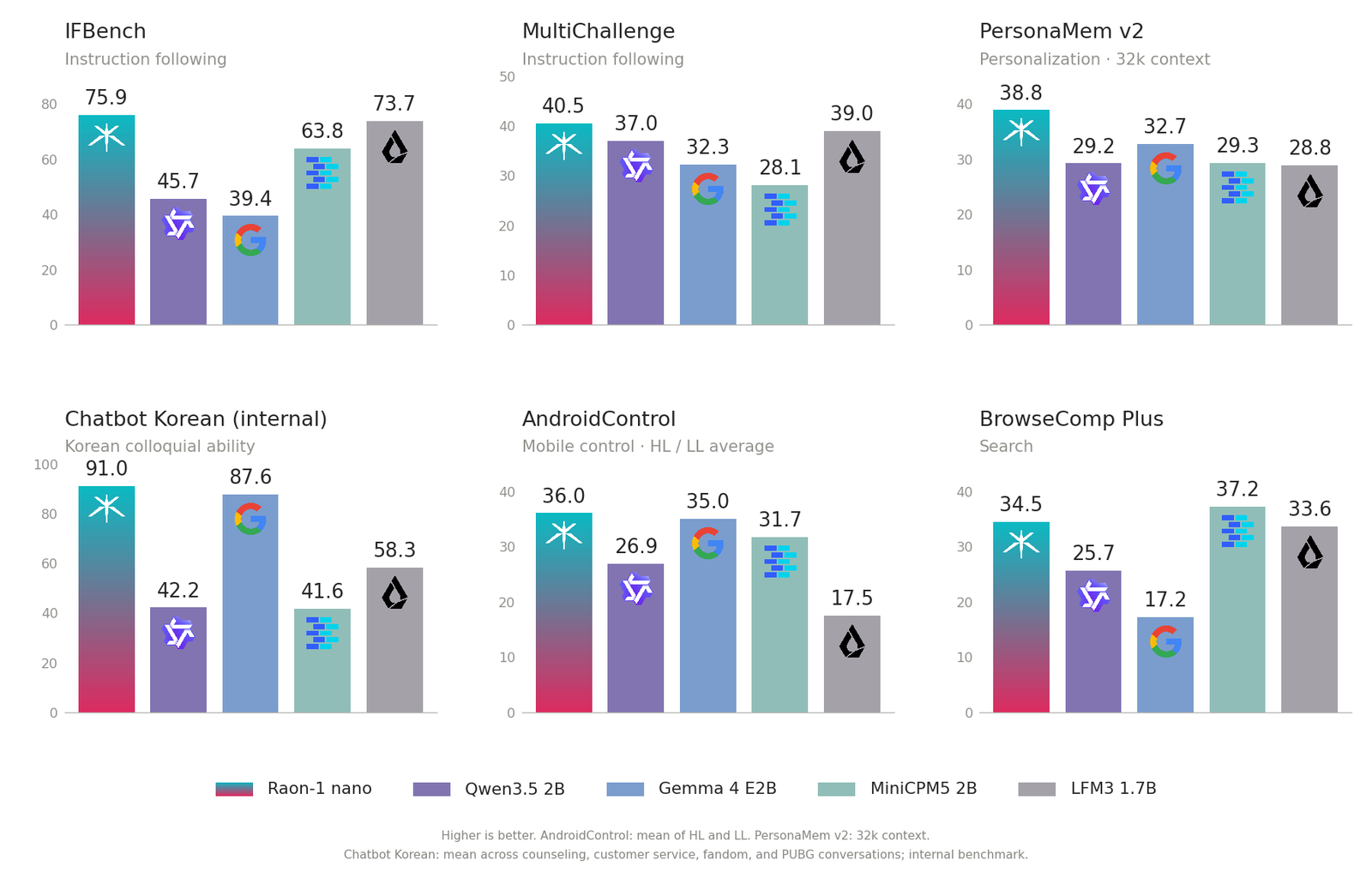
On IFBench, 75.9 over a baseline of 20 is a 55.9-tall bar; Gemma's 39.4 is a 19.4-tall one. The repo's version, from zero, is the one to read.
The post also says "Our journey from PUBG Ally toward on-device LLMs continues." That is a direction, not a deployment claim. NVIDIA's June write-up on how KRAFTON built PUBG Ally names the on-device model as Mistral-NeMo-Minitron-2B, and nothing in the Raon card says nano ships in the game. The footnote under the repo's chart does describe Chatbot Korean as a "mean across counseling, customer service, fandom, and PUBG conversations", which is a fair hint at the intended use.
KLM-1.6: 99M parameters, and its own lookup table
The same week, MinimaLabs released KLM-1.6, a 99M base model under Apache 2.0. A repost of it said "a 99M model is now #1 among all models under 250M params" and that it "beats SmolLM2-135M on every benchmark on its card".
- architecture
- KLMForCausalLM
- task
- text-generation
- library
- transformers
- license
- apache-2.0
- safetensors
- 1 shard
- largest file
- 396.1 MB
- files
- 13
- downloads
- 1.1K
- likes
- 65
- languages
- en
repo last modified 2026-11-09
The parameter count first. The single model.safetensors header sums to 98,975,308, the card's figure exactly, but
163,000 of those are not weights. They are bigram_keys (125,000 int32) and trigram_keys (38,000 int64), the hash keys
of an n-gram memory. Learned floats come to 98,812,308.
That n-gram memory is the second lookup table in this article. NgramMemory in modeling_klm.py keeps a learned
32-wide vector for each of the 125,000 bigrams and 38,000 trigrams it was built with, plus one fallback row each. For every
position it finds the bigram and the trigram ending at the current token by exact key match, projects both vectors to 512
wide, and adds the sum to the model as an extra input source that every layer's block attention residual can draw on. Like Raon's table, it adds parameters that are indexed rather than multiplied, at a scale where
it matters: 5.25M learned floats, about 5% of the model. Everything else is a tiny version of the current hybrid recipe:
24 layers, Gated DeltaNet-2 and attention at 3 to 1, hidden size 512, SwiGLU of 1,408, a 2,048-token context, and
block attention residuals.
The vocabulary is the other place the parameters went. config.json says 4,160 rows, the card says 4,100 tokens, and
tokenizer.json has 4,096 plus 7 added. Either way the embedding is 4,160 x 512 = 2,129,920 parameters. SmolLM2-135M's
is 49,152 x 576, about 28.3M. At this size a small vocabulary frees a fifth of the budget for layers, and the price is
more tokens per sentence in a 2,048-token window.
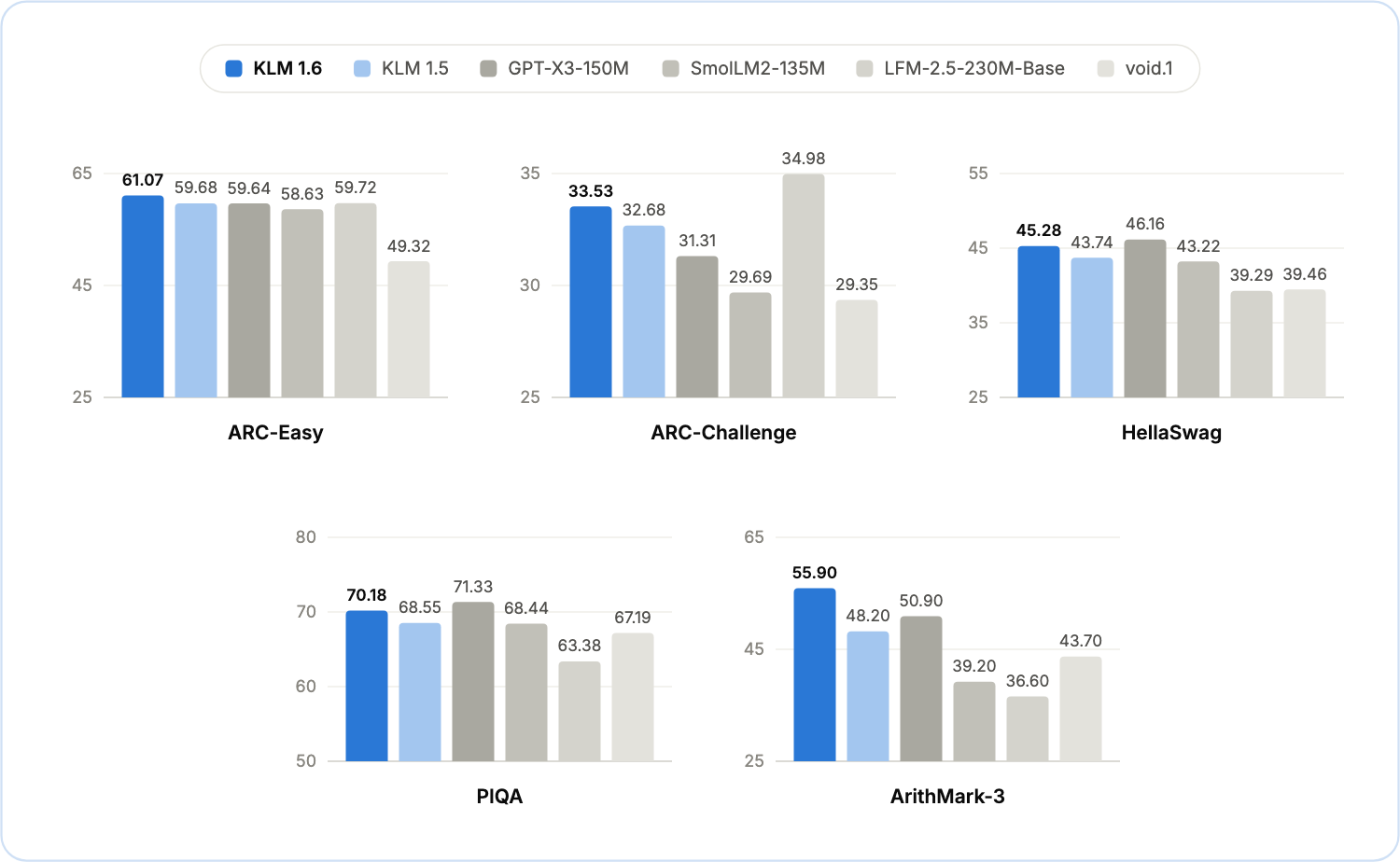
The SmolLM2 claim holds on the card: 61.07 against 58.63 on ARC-Easy, 33.53 against 29.69 on ARC-Challenge, 45.28 against 43.22 on HellaSwag, 70.18 against 68.44 on PIQA and 55.90 against 39.20 on ArithMark-3. It is not the strongest model on its own chart, though. GPT-X3-150M beats it on HellaSwag (46.16) and PIQA (71.33), and LFM-2.5-230M-Base on ARC-Challenge (34.98).
The "#1" is the Open SLM leaderboard's Intelligence
Index, a static Hugging Face space. Its formula is in index.html: rescale HellaSwag, the ARC average and PIQA so chance
is 0 and perfect is 100, add ArithMark-3 at weight 0.65, and take the weighted mean. I recomputed it for all 265 listed
models. KLM-1.6 scores 33.95. Only SmolLM2-360M (41.86) and MobileLLM-R1-360M-base (38.65) are higher, both 359M or more, which matches the card's "only two models of any size score higher". GPT-X3-150M is next at 33.05.
The board is run by AxiomicLabs, which also makes GPT-X3-150M, the model KLM just displaced, and ArithMark-3, the benchmark in the index. And the ranking turns on ArithMark-3. Drop it and the same formula puts GPT-X3-150M at 32.72 and KLM-1.6 at 32.38. KLM's arithmetic score is its biggest edge, which fits a training mix heavy on OpenMathInstruct-2 and UltraData-Math. It is also the narrowest skill on the board.
KLM-1.6 is a good small base model and an honest card. The card spells out what it is (a base model, English only, "knowledge is thin"), and it trained on a lot less: 80B tokens at constant learning rate and 100B of decay, after a warm-up that covered 128B tokens of ClimbMix for the compute of about 18B, against SmolLM2-135M's 2 trillion tokens. "Number one" is a true statement about one community leaderboard, and a soft one.
Who should run Raon-1 nano
If you are building a Korean-language assistant that has to run on a laptop, a phone-class device or a gaming PC beside a game, nano is the most interesting small model released this month, and the reason is the memory layout more than the benchmark table. 1.5B parameters of compute and a 7 KiB-per-token cache fit in an accelerator budget that a 3B dense model would not, and the other 1.6B can be paged from storage a few kilobytes per token. Use the GGUF or MLX builds; the PyTorch reference both expands the MLA cache and runs RDA in a Python loop, and the LiteRT-LM bundle is limited to 4,096 tokens and answers without thinking, which the card itself advises against.
For English tool calling I would test it against LFM3 1.7B and MiniCPM5 2B before choosing, because both beat it on BFCL v4, and MiniCPM5 also beats it on the terminal and search rows. And I would not read the release as evidence that MoE-to-dense conversion beats training a small model the ordinary way. The paper shows a better start at 4B tokens. Nano is a different, unpublished pruning of a different teacher, followed by 3T tokens and three rounds of post-training, and nobody has shown which of those steps the quality came from. KRAFTON could settle it by publishing the nano conversion and an ablation. Until then the per-layer table is the part of this release I would copy.
What was read, and what was not run
Read, with byte ranges: the safetensors headers of KRAFTON/Raon-1-nano (both shards, the tied head, the MTP module),
the first 25 MB of raon-1-nano-Q4_K_M.gguf, and the MinimaLabs/KLM-1.6 header; sampled hashes of the embedding and
LM-head tensors. Read: both config.json files; the RDA, MLA, MLP, per-layer embedding, decoder and cache code in
modeling_raon1_nano.py; nano's full card and the head of mini's; the paper's main text through Section 4.5 (arXiv v1 HTML,
with figures and key numbers checked against the v3 source), but not its appendices. Searched rather than read: the
leaderboard's index.html (its formula and model rows) and the fork's llama-arch.cpp and llama-model.cpp. Computed: every parameter split above, the cache sizes, and the Intelligence Index for all listed models.
Not run: neither model was loaded or evaluated, so every benchmark score here is the publisher's.