Open robotics mapping roundup: multi-floor SLAM, RTK in C++20, calibration checks and phone-mounted LiDAR

Five things crossed my feed in the same few days of November 2026, and they turned out to be one subject seen from five heights. A ROS 2 SLAM system that keeps a building's floors apart. A GNSS library that gets a car's antenna to centimetres. A tool that tells you whether the transform between your LiDAR and your IMU is still right. A fifty-dollar time-of-flight board stuck to an iPhone. A Livox Mid-360 plugged into an Android phone. All five are answers to the question every mapping pipeline asks before it can do anything else: where was the sensor when it took this measurement, and how sure are we?

I cloned the five repositories involved, read the parts that do the work and checked the claims against the code, the configs and the datasheets. I did not build or run any of them; where a number comes from a project's own benchmark, I say so in the sentence. The arithmetic in between is mine, and the two widgets below are toys I wrote to show the mechanism, not ports of anyone's solver.

If you work on LiDAR SLAM, the first section is the one to read: StrataSLAM's answer to perceptual aliasing is a structural one, and it is more interesting than its README makes it sound.

StrataSLAM keeps one map per floor and refuses everything else

StrataSLAM is a multi-floor 3D SLAM system for ROS 2 Jazzy from José Miguel Guerrero at Universidad Rey Juan Carlos, released as v0.2.0 under Apache-2.0 at the start of November (the citation file says 2 November; the repository was created on 3 November and had 41 stars when I looked on 12 November). It takes an RGB-D camera, a 3D LiDAR, both, or a 2D laser scanner, with an IMU, a barometer and wheel odometry as optional extras, and it writes one point cloud per floor plus a global one. The README's one-line pitch is "one point cloud per floor and a global one, without the floors collapsing into each other". I read it at commit ec705b1 (10 November).

Why identical floors collapse

Loop closure is the step that makes SLAM more than odometry. The front end proposes "I have been here before" by comparing a descriptor of the current scan or image against a database of past keyframes: a Scan Context ring descriptor for LiDAR, a bag of visual words for a camera. A verification step registers the two scans, and if the fit is good, the back end adds a relative-pose factor between the two keyframes and re-solves the graph. That factor is precise. Two scans of the same corridor registered with GICP agree to a few centimetres, which is exactly why one good loop closure can pull a whole drifted trajectory back into shape (the GTSAM article has a loop you can close by hand).

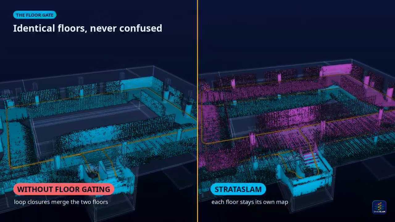
Now put the robot in an office block where floor 2 has the same corridor, the same doors and the same lift lobby as floor 1. The place recognizer is doing its job when it says floor 2's lobby looks like floor 1's lobby: the descriptors are the same because the geometry is the same. Verification passes too, because the scans really do register. The back end receives a precise, internally consistent, completely wrong constraint saying two keyframes three metres apart vertically are the same place. Repeat that at every lobby and corridor, and the optimizer does the only thing least squares can do: it moves floor 2 down onto floor 1, because dozens of centimetre-precise loop factors outvote one sloppy stair measurement. That is perceptual aliasing, and it is a failure of the problem formulation, not of any component.

You can watch it happen in a stripped-down version. Floor 1's height $h$ is the only unknown. The stairs say $h = 3.0$ m with $\sigma = 0.15$ m, which is the z standard deviation StrataSLAM assigns to a stair or ramp transition (its ADR-0015). Every accepted cross-floor loop says $h = 0$ with the registration's $\sigma_\ell$. The least-squares estimate is a weighted mean:

With $\sigma_\ell = 0.05$ m one false loop has weight 400 against the stairs' 44.4, so it already outvotes the stairs nine to one and puts floor 1 at 0.30 m. A barometer at $\sigma = 0.05$ m slows the slide, since it adds a second honest vote, but it is one vote, and the loops keep coming.

The widget's default is the number StrataSLAM's own negative control produces. Scenario S04 is S03 (two identical floors joined by stairs, camera only, no IMU) run with the floor gate switched off by a debug flag. Its report in docs/scenarios.md lists 41 accepted loops, 35 cross-floor candidates, one floor instead of two, an ATE of 1.46 m and a collapse rate of 0.853659. The collapse rate in metrics.cpp is the share of accepted loops whose two ends are on different floors, and 35 / 41 = 0.853659, so every one of the 35 cross-floor candidates was accepted, alongside six loops on the right floor. With the gate on (S03, same building, same seed) the run has 8 loops, all on-floor, two floors, an ATE of 0.022 m and zero cross-floor candidates. Zero candidates, not zero accepted: with the gate on, the recognizer never even proposes one, for a reason that comes up below. The test harness fails the run if the negative control does not collapse, which is the right way round: a test that cannot see the bug cannot prove the fix.

Noticing that you changed floor

Refusing cross-floor loops only works if every keyframe carries the right floor label, so most of StrataSLAM's complexity is in floor_manager.cpp (843 lines), a state machine that decides when the robot has left a floor and where it arrived. Any of three signals can open a transition:

• Odometry height. The tracked altitude moves more than depart_dz = 0.30 m from the floor's reference height.
• Barometer. The filtered pressure height moves more than 0.50 m.
• IMU. The trimmed one-second mean of gravity-free vertical acceleration exceeds 0.25 m/s² for half a second while the odometry sees no vertical motion. The trimmed mean drops the top and bottom 20 % of samples, because a wheel hitting an edge reads tens of m/s² for one sample, and walking bobs average out.

The IMU path is for elevators, where the camera or LiDAR sees a cabin that moves with it and reports no climb at all. The transition closes after two seconds of calm, and is then classified:

• Elevator if the barometer moved at least 1.0 m while the odometry moved less than half of that; or, without a barometer, if the IMU's double-integrated height is at least 1.0 m with the odometry static. The double integration uses a zero-velocity update at the end (the cabin is at rest again), spreading the residual velocity linearly over the ride, which removes most of an accelerometer bias.
• Aerial if the platform is a drone, or the horizontal run was under half the climb.
• Ramp or stairs otherwise, split on the median slope over 1 m windows of the climb: under 15° is a ramp.

The height change is then snapped to a level. With the default floor_height_prior of 3.0 m, a change counts as a floor only when it is within 0.4 of a whole number of storeys, which is how the half-way landing of a U-shaped stair is kept from becoming a floor. Matching an existing level uses a tolerance of 0.4 times the prior (1.2 m), widened by the level's own uncertainty; an elevator ride measured by the IMU is trusted to 5 % of its height. Those numbers came from real data: the comments cite sequences from the Elevator-VIGS dataset by name, such as an "Office4" run that rode 14.75 m up and walked 15.43 m down the stairs, ended 0.68 m off, and opened a phantom third level before the 5 % term was added. That run had no height prior, so the tolerance was 0.4 times the 1.5 m minimum change, 0.6 m, not 1.2 m. A plateau rule (20 s calm while travelling 10 m) also accepts a mezzanine that is no multiple of 3 m.

Three layers of refusal

The floor gate is three independent checks, and the code names them:

1. Per-floor place recognition. Each floor has its own Scan Context database and its own bag-of-words index (scan_context.hpp: "the caller owns one instance per floor (gating layer 1)"). A query only searches the current floor, so a keyframe on floor 2 is never compared with floor 1. This is why S03 reports zero cross-floor candidates.
2. Label check. Backend::verify_loop_allowed rejects a loop whose two keyframes carry different floor labels, or any keyframe without a label.
3. Graph membership. There is a separate factor graph per floor, and FloorGraph::add_loop refuses a factor to a node it does not hold. ADR-0040 records that the original layer 3 just re-compared the labels, so a mutation test could delete it unnoticed; it was rewritten to check what the factor actually joins.

The consequence is stronger than "we filter false loops". No online code path can write a cross-floor factor, so the failure in the widget cannot happen however similar two floors look. What can still go wrong is the floor label itself: a missed transition maps two floors into one graph, and a phantom transition splits one floor in two. Every hard case in the floor manager's comments is one of those.

Putting the floors back together, offline

Each floor is then a separate map with its own frame, and the building has to be assembled. strataslam fuse does it offline in a gravity-aligned four-degree-of-freedom group, $\mathrm{SE}(2)\times\mathbb{R}$: yaw, $x$, $y$ and $z$, with roll and pitch fixed by gravity. The documentation in docs/math/pose4.md follows Solà, Deray and Atchuthan's micro Lie theory notation. A pose $X = (\theta, \mathbf t)$ composes as

which is SE(2) with a free height bolted on. The constraints between floors are the transition records (the relative pose measured across the stairs or the ride, with a covariance that grows 3 % per metre the odometry travelled), the barometer, user-placed anchors, a weak floor-height prior with $\sigma$ = 0.10 m, and a structural registration that correlates rasterised wall slices of two floors.

That last one is where aliasing comes back, and the project handles it honestly. Registering two floors by their walls cannot tell one level seen twice from two identical levels stacked. ADR-0027 reports that on a Gazebo garage with near-identical floors, every pair was declared ambiguous (best score 0.996 against a runner-up of 0.97) and contributed nothing, which is the correct outcome. ADR-0031 adds "same-level candidates": pairs of floors whose structure matches and whose heights differ by under 2 m are listed as warnings and never applied. On one real bag it listed three candidates, one of them right. The user confirms which with --same-level. A candidate list is advice, not a classification, in the ADR's own words.

expand

What the evidence covers

The fifteen synthetic scenarios run on 20 seeds each, and docs/results.md reports every failure with its seed: S07 (an elevator with no IMU or barometer, fused with anchors) passes 13 of 20 on a 0.10 m translation bound; S13 (a 2.9° ramp) fails once at 0.2512 m against 0.25 m. S15, four identical floors up by elevator and back down by the stairs, passes but with a mean floor-height error of 0.4507 m. Read the simulator results with ADR-0017 in mind: the camera is simulated at feature level, as keypoints with descriptors and depth, not rendered images, so the visual front end's real failure modes are not in them.

The real-data evidence is thinner and is said to be. On TUM RGB-D fr1/xyz and fr2/xyz the visual odometry gets 0.0143 m and 0.0152 m ATE. On KITTI drive 0027 (692 m) the full LiDAR pipeline gets 0.40 m ATE with one loop closure at 52 ms a scan on one thread. The multi-floor claims rest on Elevator-VIGS: ADR-0059 reports that on its 16 real sequences one-way rises land within 0.06 to 0.9 m of the truth and round trips close within 0.07 to 2.6 m. The structural floor registration has, per ADR-0027, "not yet contributed a constraint" on real data. None of that undercuts the gate: refusing cross-floor loops does not need a benchmark to be correct. It does mean the hard part, labelling floors correctly on a real robot in a real stairwell, has been tested on far fewer buildings than the scenario table suggests. A multi-floor equivalent of the Hilti SLAM datasets, graded against surveyed points, would settle it.

Forty-one stars and a week old, with 69 ADRs (each deviation from its own plan written down with a reason), a negative control in CI and mutation testing on the gate. I would try it on a multi-storey capture before I would trust a single-graph SLAM system to keep two identical car-park levels apart.

libgnss++: from a thirty-metre guess to a centimetre fix

libgnss++ is Ryohei Sasaki's C++20 GNSS toolkit (MIT, 260 stars on 12 November, read at 1f7bd1e, version 0.6.0). It implements single-point positioning (SPP), real-time kinematic (RTK), precise point positioning (PPP), Japan's CLAS and MADOCA correction services, RTCM, UBX and QZSS L6 decoding, a GTSAM-backed GNSS/IMU factor graph, Python bindings, a ROS 2 player and a WebAssembly build that runs gnss solve in a browser tab. Its src/ directory alone is about 104,000 lines. It is a lot of library, and the core of it is two pieces of estimation worth understanding.

Pseudoranges and four unknowns

A receiver measures, for each satellite $s$, a pseudorange: the signal's travel time times the speed of light, biased by the receiver's clock.

The satellite position $\mathbf p^s$ and clock $\delta t^s$ come from the broadcast ephemeris, the ionospheric delay $I^s$ and tropospheric delay $T^s$ from models. That leaves four unknowns: the position $\mathbf x$ and the receiver clock bias $c\,\delta t_r$. Linearise around a guess $\mathbf x_0$, with $\mathbf e^s$ the unit vector from receiver to satellite, and each satellite gives one row of a linear system:

Iterate until $\Delta$ stops moving. Four satellites determine it, more over-determine it, and $W$ down-weights low satellites whose signals cross more atmosphere. spp.cpp is this loop (3,007 lines once you add multi-constellation clock offsets, robust re-weighting and satellite exclusion modelled on MRTKLIB's estpos), starting cold from a seed about 24,000 km out. The answer is good to a few metres, limited by the code measurement's noise and the atmosphere models.

Carrier phase and the integer problem

Centimetres need the carrier phase. The receiver tracks the phase of the 1575.42 MHz L1 carrier, whose wavelength is $\lambda = c/f$ = 0.1903 m, to a small fraction of a cycle. But it only knows the fractional part when it locks on: the whole number of cycles between satellite and antenna, $N^s$, is unknown.

RTK removes almost everything else by differencing. Subtract the base station's measurement from the rover's (the satellite clock cancels), then subtract a reference satellite's single difference from each other satellite's (the receiver clocks cancel). Over a short baseline the atmosphere is nearly the same at both receivers and cancels too:

What is left is the baseline $\mathbf b$ and one integer per satellite pair. In libgnss++, as in RTKLIB, an extended Kalman filter carries the baseline, velocity, optional ionosphere terms and one single-difference ambiguity per satellite and frequency; rtk_filter.cpp forms each double-difference phase row from two of those states ($\lambda_\text{ref} N_\text{ref} - \lambda_s N_s$). The filter's ambiguities are real numbers, the float solution, with a covariance $Q_{\hat a}$. Snapping them to integers is integer least squares:

Rounding each $\hat a_i$ on its own is wrong whenever the ambiguities are correlated, and double differences always are: they share the reference satellite, and over a few seconds the satellites barely move, so $Q_{\hat a}$ is a long, thin, tilted ellipse. Teunissen's LAMBDA method decorrelates first, with an integer, volume-preserving transform $Z$ (built from integer Gauss transforms and permutations of an $LDL^\top$ factorisation), so the search in the transformed space is small, then maps the answer back with $Z^{-\top}$. libgnss++'s lambda.cpp says at its head that it is "Ported line-by-line from RTKLIB's lambda.c" (BSD-2-Clause, T. Takasu), with Eigen in place of C arrays. That is a good choice: it is the most exercised LAMBDA in open source, and the README's "without an external RTKLIB runtime" is true while the heritage is plain.

The search returns the best and second-best integer vectors with costs $q_1 \le q_2$. The ratio test accepts the best only if

with $\kappa$ = ambiguity_ratio_threshold = 3.0 by default (rtk.hpp). Optional modes make it 1.5 with 20 or more satellites, 2.0 with 15 or more, 2.5 with 10 or more, and 2.0 while an ambiguity is being held after a run of fixes. There is also a fixed-failure-rate ratio table from Hou, Verhagen and Wu (Sensors 2016) and partial fixing of a subset. Once the integers are accepted, the baseline is conditioned on them, $\check{\mathbf b} = \hat{\mathbf b} - Q_{\hat b \hat a} Q_{\hat a}^{-1}(\hat{\mathbf a} - \check{\mathbf a})$, and the same formula appears as xa = head_state - sQab * slv.solve(sf - sx) in rtk_ar_resolve.cpp.

The toy shows the three regimes. With few epochs (noise run 3, four epochs), rounding picks (1, 1) while integer least squares already finds (0, 0), because it measures distance along the ellipse. Run 2 at one epoch is the dangerous one: the best integer is (−3, −2), wrong, and its ratio is 3.1, so a threshold of 3.0 accepts it. A wrong fix is worse than staying float, because the solution then reports centimetre confidence about a position that can be off by a wavelength per satellite; that is why the PPC tables below count wrong fixes separately.

What the benchmark tables say, and what they do not

The README leads with that Odaiba animation: median horizontal error 0.38 m against RTKLIB demo5's 7.41 m over 172 common epochs. The README itself says it is "a favorable selected segment, not a full-run benchmark", and the hero's notes (docs/odaiba_hero.md) record a correction made on 26 October: an earlier version ran RTKLIB GPS-only by a config mistake, and with every constellation RTKLIB fixed 147 of that window's 201 epochs, so the window was re-selected. On the full drive the honest comparison is the "Urban RTK" row: with --preset urban, 7,467 fixes against demo5's 5,839 with fewer wrong fixes, while the default profile fixes only 1,298 epochs.

The PPC 2024 table (six Tokyo and Nagoya runs) reports a macro fix rate of 70.939 % against 54.326 % for gici-open, with 1.463 % wrong fixes. Two caveats are printed next to it: these are "in-sample benchmark results, not a held-out generalization claim", and gnss reproduce ppc-goal rescores 26 frozen tier inputs whose solver commands were not recorded, so the table "cannot be regenerated from scratch". The Smartphone Decimeter Challenge score of 0.714 m private is a late, unranked submission reached after per-drive Kaggle probes, again as the README states.

expand

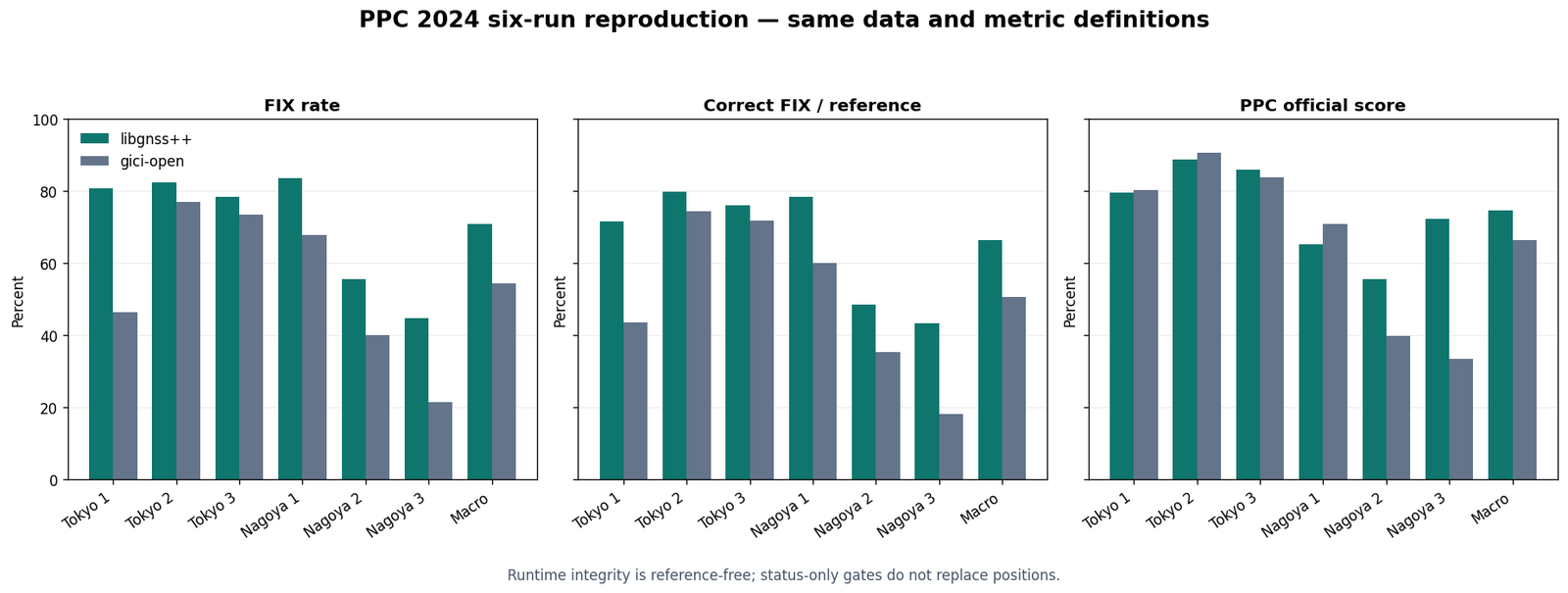
I like this README more than most because it publishes its own corrections. It also has the shape of a project tuned against the benchmarks it reports, with an AGENTS.md at the root and docs named like work packages. For a positioning engineer the library's value is the RTKLIB-compatible core in modern C++ with a factor-graph back end beside it, not the leaderboard rows.

Calibrex checks a calibration instead of trusting it

Calibrex, from the same author (Apache-2.0, 62 stars, read at 2f9d8d0 on 12 November, labelled alpha), starts from a question most calibration tools skip. You calibrated the rig once. Is the transform in /tf_static still right after someone remounted the IMU? It has three commands: calibrex estimate reads a bag and estimates each sensor pair's transform from the motion alone, with no target; calibrex check compares a deployed calibration against that estimate on another recording; calibrex drift asks whether it changed across bags. It reads rosbag2, MCAP and ROS 1 bags without a ROS install, and covers IMU-LiDAR, camera-IMU, camera-LiDAR (rotation only), LiDAR-LiDAR, GNSS lever arms and vehicle frames.

The IMU-LiDAR rotation solver shows the method in one equation. Between consecutive LiDAR odometry poses $R_i$ and $R_{i+1}$, the mean angular rate in the LiDAR frame is $\boldsymbol\omega_L = \mathrm{Log}(R_i^\top R_{i+1})/\Delta t$. The gyro measured the same rotation in its own frame, shifted by a clock offset $\delta$ and biased by $\mathbf b$:

Calibrex initialises $R_{LI}$ with a weighted Procrustes alignment of the two sets of rates (so any mounting works), then solves for rotation, offset and bias with a nonlinear least squares in which the interval means of the gyro come from a cumulative trapezoid integral. Rotation about an axis is only observable if the recording rotates about the other axes: a car that only yaws says nothing about the yaw of its IMU mount.

The lever arm (translation) is harder, and the docs explain why. It enters only through rotation: $(R_j - R_i)\,\mathbf l = R_i(\mathrm{Exp}(\boldsymbol\theta) - I)\,\mathbf l$, so the information on axis $a$ scales with the rotation perpendicular to $a$. A planar vehicle can see the horizontal components of a GNSS antenna's lever arm from its turns, and never the vertical one. When an axis is not observed, Calibrex writes it as NOT MEASURED instead of inventing a number.

The verdict is a rule you can audit in check/verdict.py. For each judged axis with error $\delta$ between the deployed transform and the estimate, the tolerance is $\max(3\sigma, \text{floor})$, with a floor of 0.5° for rotation and 0.02 m for translation. The axis passes if $|\delta|$ is within the tolerance, fails beyond twice it, and warns in between. An axis the data did not observe is listed as unchecked, and a pair with no judged axis at all is "inconclusive".

expand

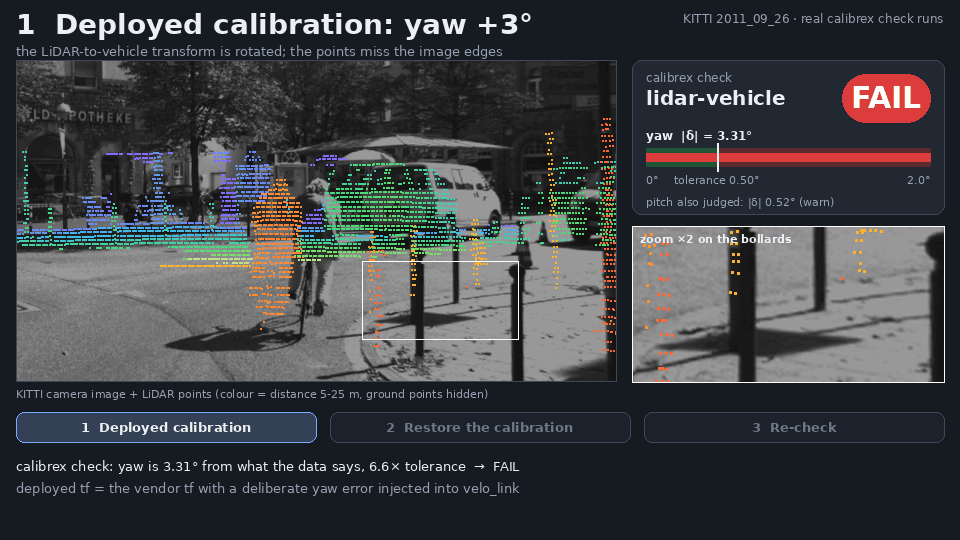
That frame checks against the rule: 3.31 / 0.50 = 6.6, beyond the factor of 2, so fail; the pitch error of 0.52° is between 0.50° and 1.0°, so warn, which is what the panel prints. The README's other demos are all on public data with their own numbers: a second Ouster on NTU VIRAL snapping from a 19.1 cm to a 4.4 cm median point-to-plane residual (the design value gives 4.6 cm), and camera-IMU on Hilti 2022 landing 0.45° and −0.21 ms from Kalibr's target-based result. On camera-LiDAR, the README says the check flagged 23 of 27 perturbed candidates and never flagged the unmodified reference, and calls that development evidence, not a claim.

The deskew clip is the clearest argument for caring. A Mid-360 sweep takes 100 ms; at 180°/s the head turns 18° during it, and every point has to be moved to one instant using the IMU, which is only as good as the IMU-LiDAR rotation and time offset. The same deskew happens at the start of FAST-LIO2; a wrong extrinsic there smears every scan before the filter ever sees it. A tool that tells you, per axis, that your extrinsic has moved by more than the data's own noise, and also tells you when your recording could not have detected it, is the kind of thing I would put in a fleet's nightly checks.

Fifty dollars of time-of-flight on an iPhone

On 10 November Laan Labs posted a short video: "Testing 3d scanning with this ~$50 lidar sensor (ST VL53L9CX) attached to an iPhone. Works pretty well for quick indoor scans using just ARKit poses." It had about 67,000 views two days later, and @taziku_co, the CEO of the Japanese studio taziku, reposted the same video the next day under a line that translates as "how far can 3D scanning go with a roughly $50 small LiDAR and a phone?".

The sensor is ST's VL53L9CX, and its datasheet (DS14879 Rev 7, July 2026, included in the board's repository) is specific. It is a direct time-of-flight module: two 940 nm VCSELs flood the scene, and a SPAD array (single-photon avalanche diodes) times the returning photons. Distance is $d = c\,t/2$, so one nanosecond of round trip is 15 cm, and the module gets its accuracy by building a histogram of photon arrival times over many pulses per zone and finding the peak on chip. The specs:

• up to 54 × 42 zones (2,268 depth values a frame), with binned modes down to 4 × 4;
• 55° × 42° field of view, 71° diagonal;
• ranging from under 5 cm to 8.8 m in its precision mode;
• up to 100 Hz in some profiles; the datasheet's example profiles run full resolution at 100 fps for a short 5 m range, 30 fps for 8 m;
• accuracy in precision mode at full resolution, indoors, under 8 mm below 1 m and under 0.5 % beyond, on a 17 % grey target;
• a 12.8 × 6.1 × 4.6 mm module.

The resolution is the number to keep in mind. 55° across 54 zones is about 1° per zone, so at 3 m one depth value covers about a 5 cm square of wall. That is a coarse depth camera, not a scanning LiDAR, and it explains how the scans look: good room shape, soft edges on everything small.

The board is Remi De Coster's USB-LiDAR-VL53L9 (MIT for his hardware and code, 136 stars, read at 39a2dd4). It is a 34 × 30 mm KiCad 10 PCB with the VL53L9CX, an ST LSM6DSV16BX 6-axis IMU and an STM32C552 Cortex-M33 that enumerates as a USB CDC serial device.

expand

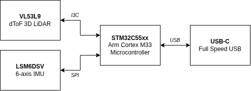
The firmware does very little on purpose. It triggers a frame, polls the ready flag every 500 µs, reads the raw 14,842-byte frame (a _Static_assert pins the size for binning 2) into one of two ping-pong buffers and ships it in a framed packet with a sequence number, a microsecond timestamp and a CRC-32. The README measures about 35 frames a second and 520 kB/s; 14,842 bytes times 35 is 519,470 bytes a second, so the two agree, and that is about a third of USB Full-Speed's 12 Mbit/s. IMU samples go out at 120 Hz in the same stream. Depth is not computed on the board: the host turns raw frames into depth with ST's processing library and the sensor's factory calibration, which the bundled web app compiles to WebAssembly. That library is under ST's SLA0111 licence, for use with ST sensors only, so the pipeline is open hardware with a closed-source step in the middle. That is normal for ST's ToF parts and worth knowing before you plan to port it.

expand

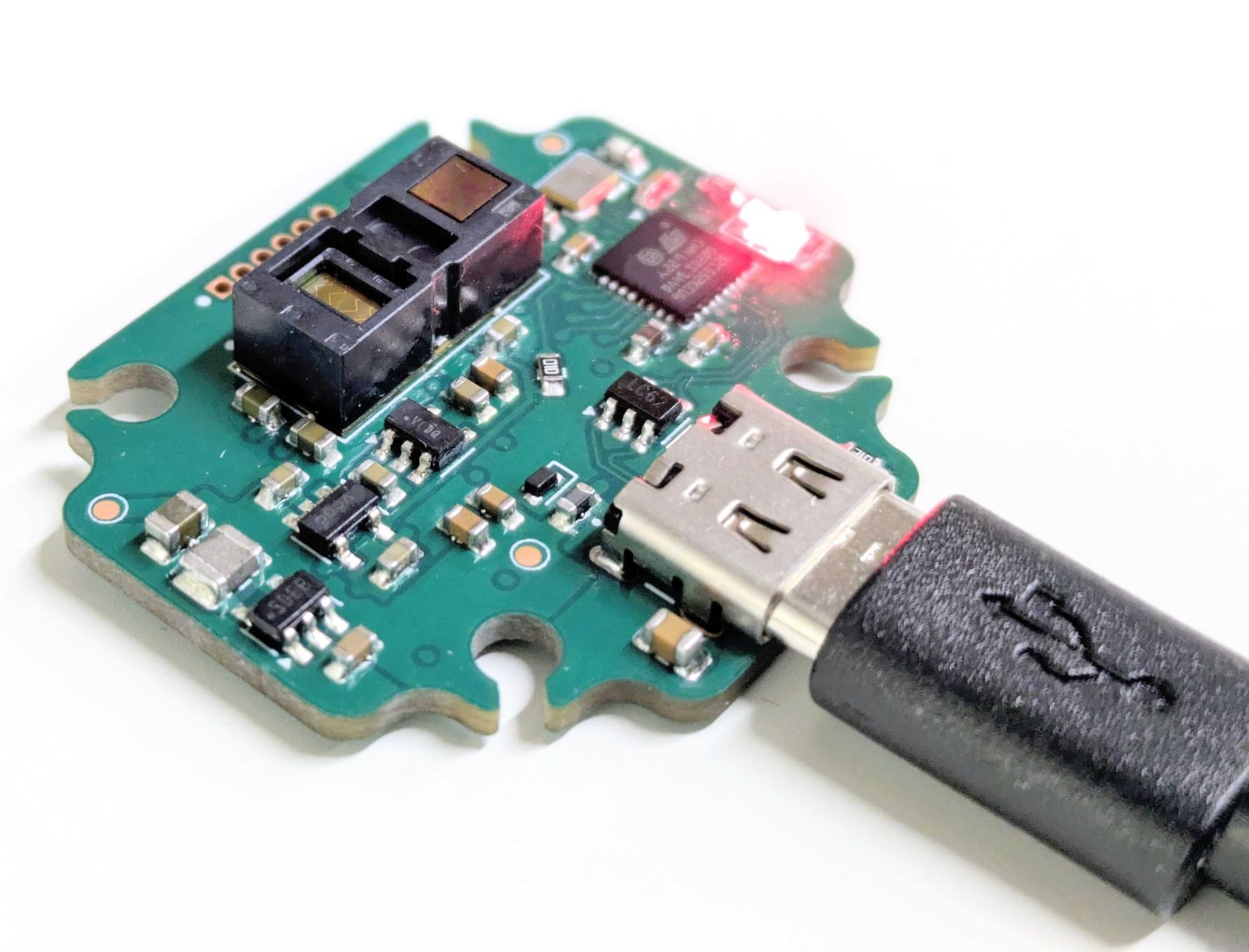
Laan Labs' iPhone app is not in that repository and has not been published, so what follows is only what the video and their replies show. The app's status line reads "VL53 → mesh · edges off · 54x42 · 15 fps", so it ran full resolution at 15 frames a second, 34,020 depth values a second. The pose comes from ARKit, Apple's visual-inertial odometry, not from the ToF sensor; the sensor contributes depth only. That is the easy half of mapping: with poses given, fusing depth frames into a volume or mesh is a solved problem, and the scan's quality is bounded by ARKit's drift and by how well the depth frames are registered to the phone's camera. In the replies, Laan Labs said indoor results look similar to the iPhone's own LiDAR, the iPhone's works much better outdoors, and the VL53L9CX "might have a bit more range indoors", adding that the iPhone pipeline also has ML depth upsampling this demo does not. Two people asked the questions I would ask: how the sensor's timestamps are synced to ARKit, and how the extrinsic to the camera was calibrated. Neither had an answer among the replies I could fetch through a mirror on 12 November. Both are exactly the IMU-camera problem Calibrex measures, at the scale of a phone case.

The "~$50" is Laan's figure. The repository's bill of materials lists parts and Digi-Key numbers but no prices, so I cannot check it; the author says he is only exploring selling assembled units.

A Mid-360 on an Android phone, and a link that is not about it

The other phone post is from @sm0219370893504 (schan, CTO of IndustryAlpha), also on 10 November: lately he has been playing with 3D point clouds everywhere, DOOM-style, "so for now I connected a phone to a mid360 and did 3D SLAM" (my translation from the Japanese). In the replies he confirms the sensor is a Livox Mid-360, "a compact 360° 3D LiDAR with a built-in IMU".

The 11.6-second clip is a phone on a table, with an Android navigation bar, so not an iPhone. Its status chips read "Ethernet", "Mid-360 145k点/s" and "IMU 200Hz", and a counter shows 37,844 points four seconds into a map. The Mid-360's spec page lists 200,000 points a second, a 360° × 59° field of view (−7° to 52° vertical), 40 m range at 10 % reflectivity, a built-in ICM40609 IMU, 100BASE-TX Ethernet, 265 g and 6.5 W from a 9 to 27 V supply. My reading, not something the post says: the phone talks to the LiDAR over a USB-Ethernet adapter, the LiDAR runs off its own supply, and the phone does the computing.

The post names no SLAM algorithm and links no code. A LiDAR with a built-in IMU and a scan pattern that never repeats is the textbook input for a tightly coupled LiDAR-inertial odometry like FAST-LIO2, and running one on a phone-class ARM SoC at a Mid-360's rate is plausible, but that is my guess, not something the post says.

One reply under it linked Foadsf/parallax, and it reads as if it might be related. It is not. The same account posted the same link under Laan Labs' video ("What if you wouldn't need extra hardware?"). Parallax (GPL-3.0, created 2 November, read at a1bc267) is an Android app that does photogrammetry on the phone: RootSIFT features, five-point RANSAC, incremental structure from motion with a Schur-complement bundle adjustment that self-calibrates each lens and models rolling shutter, then semi-global matching for dense stereo, with metric scale from two rear cameras' factory baseline or a printed ArUco marker. A case-insensitive search of the repository for "lidar", "livox" and "mid360" finds nothing. It is a reasonable piece of work about a different problem, camera-only object scanning, and it has nothing to do with the Mid-360 post.

Where this leaves a LiDAR person

The two phone demos are the fun ones and the least informative. Both delegate the hard part: Laan Labs to ARKit, schan to an unnamed odometry on hardware that costs more than the phone. Both are still the right demos to build. A 54 × 42 zone sensor at fifty dollars that ranges 8.8 m indoors is a real new option for close-range fill on a capture rig, next to the survey-grade heads in Hesai's Kosmo or the 360-camera rigs in Gaussian-splat capture in practice, and the VL53L9CX board is the cleanest way I have seen to get raw frames off one, licence caveat and all.

libgnss++ is a serious library with honest documentation and benchmark claims you should treat as the author's own tuning, which the author says. Its RTK core is RTKLIB's mathematics in modern C++, and the widget above is how that core decides when to believe itself.

Calibrex and StrataSLAM are the two I would actually spend time on. They share a habit: each refuses to output something it cannot support. Calibrex will not write a lever-arm axis it did not observe. StrataSLAM will not write a factor between two floors, and lists "these two floors might be the same level" as a warning for a human rather than applying it. Aliasing on repeated floors and drifted extrinsics share a nasty property: the map comes back wrong while every residual looks fine. Both projects attack them by making the wrong answer impossible to write down, rather than by making the estimator cleverer. That is the right instinct. StrataSLAM still has to prove its floor labelling on more real buildings than Elevator-VIGS and a few Summit bags, and I would want to see that before putting it in front of a customer. The gate itself I would take today.