2026-11-09 · 36 min · looped-transformers · mixture-of-experts · interpretability · routing
Why read this
Hightop 30%Walks LoL's forward pass and router code, checks its MoE match, and runs 53 CPU toy runs: given routing transfers, five learned-router schemes do not.
- Interactive explanations
- Original analysis
- Runs on a laptop CPU
LLM architectureMITResearch paper
How this was scored
- Is it new?
- 2 of 3: A real new idea, method or capability
- Can I trust it?
- 2 of 3: Measures key facts from files, code or configs
- Can I run it?
- 2 of 3: Open code or weights with real limits
- Will I understand it?
- 3 of 3: Mechanism carried by interactives built from real code or data
- Can I act on it?
- 2 of 3: A concrete recipe, numbers or comparison
- Will it last?
- 2 of 3: A reference for a year or more
- Does it affect many?
- 1 of 3: A specialist community
- Only here?
- 2 of 3: A teardown or measurement few others did
Score 71 of 100, ranked 117 of 701 rated articles. Each question is answered 0–3 by hand, and a 3 is rare. How articles are scored
Micah Goldblum's thread opens with the pitch: "Programmers build wildly different algorithms by chaining the same few primitives in different orders. LLMs can't: every input runs through the same layers in the same order." The paper behind it is Library of Layers (LoL) (arXiv 2611.03526, Rahmani, McLeish, Li, Lotfi, Frossard, Goldblum; EPFL, NYU, Columbia, Maryland), and the code is at arahmani1/library-of-layers under MIT.
The model keeps a shelf of transformer blocks. At every depth of its middle section, a small router picks which block runs next. Different windows of text can take different paths through the same shelf, and the same block can run twice or not at all.
I wanted to answer three things:
- How is the order chosen? A learned router, a search, or RL? (A router. It is an MoE gate with top-1 selection.)
- Do the paper's runs match its text? (Mostly. A few configs differ from what the paper says, listed below.)
- Does a learned order actually behave like composing primitives? For this I trained a small version on CPU on a task built from four primitive functions, then went back for a second round: a rerun under different optimiser settings, an ablation of which kinds of routing transfer, and five ways of training the router.
Short version: the mechanism is clean and the routing paths it learns are readable and steerable, as reported. In my toy, a router that has to learn the order on its own did not find the primitives, under any of five training schemes. Giving the model the right routing did help on unseen combinations, by less than my first round suggested, and the routing that helped most reused no block across depth at all. That gap is the interesting part.
- license
- MIT
- branch
- main
- tests
- none found
- source
- 785.7 kB
- commit date
- 2026-11-03
by size of tracked source at this commit, file counts in brackets; docs, data and vendored trees excluded
local clone, 2026-11-10 at be07d22 — branch, commit, commitDate, fileCount, hasTests, languages, license, licenseFile, shallow
shallow clone: counts describe the pinned tree, not the history
What a "library of layers" is
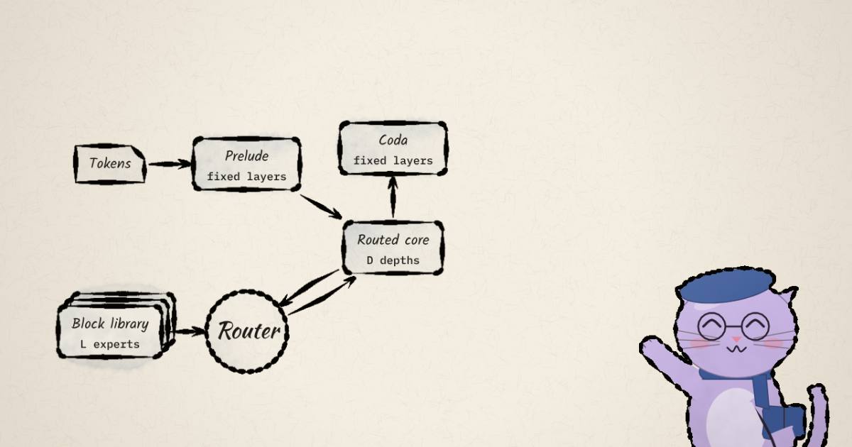
A LoL model has three parts (paper, Section 3.1):
- a prelude : a few ordinary transformer layers with full causal attention;
- a routed core: routed depths, each of which runs one block chosen from a library ;
- a coda : a few more ordinary layers, then the LM head.
counts blocks stored; counts blocks executed. With and , a window might run , repeating one block and skipping another. The paper calls that sequence a routing path, and each library block an expert.
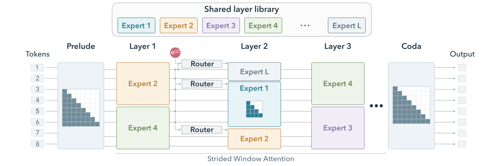
This is not mixture of experts in the usual sense. A standard MoE layer routes each token to a few of that layer's MLPs, and layer 7 always runs before layer 8. In LoL, every depth draws whole blocks (attention and MLP) from one global pool. So routing decides which computation runs and in what order. Looping, as in Huginn and Ouro, is the special case where the path is fixed and repeats one block.
The forward pass, term by term
The paper's Algorithm 1 is short enough to write out whole. Take a sequence of tokens and width . The prelude runs first, with full causal attention:
Then, for each routed depth , five steps.
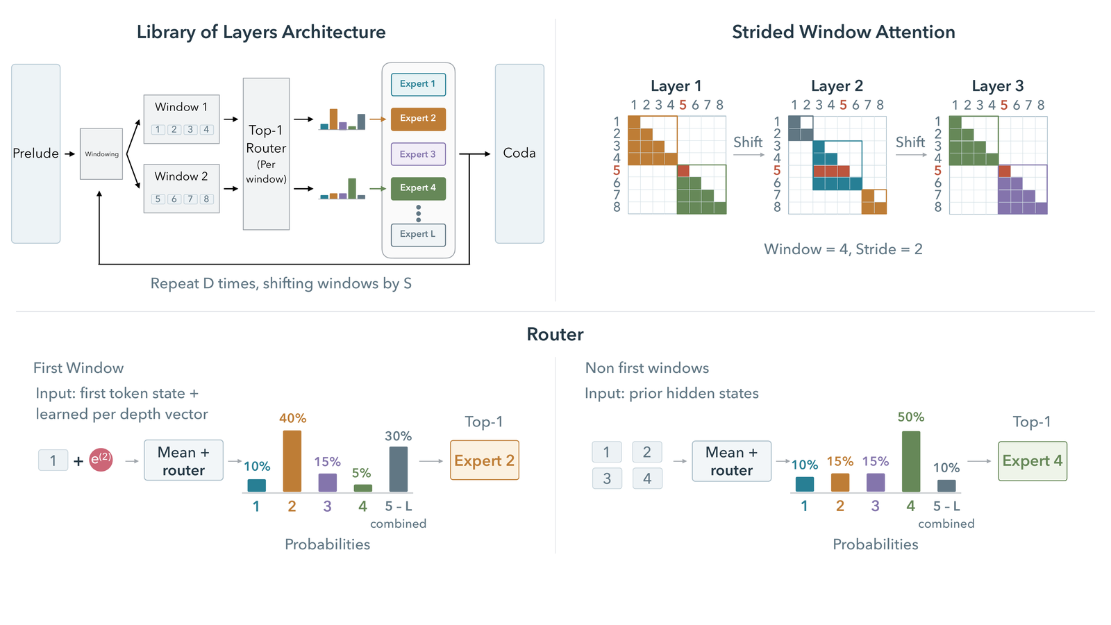
1. Cut the sequence into windows. With window size and stride , the boundaries shift by , and window is . With the natural-language settings (, , ), odd depths have 8 windows of 128 tokens. Even depths have 9: a half window of 64 at each end and seven full ones between (reasoned from the formula).
2. Summarise what came before. Each window's mean hidden state is . The router's input for window is the mean of the earlier windows' means:
is a learned vector per depth, and is the window's first token. The code computes with a cumulative sum over windows that restarts at each document boundary (RouterInputEncoder.build_features). Note what is not: it never looks at window itself. The block that runs on a window is chosen from its past. That is what keeps generation causal, and it is why the route for a window is fixed before its first token is generated.
3. Score the library. The router is one linear layer, . In training, the code adds noise whose scale is itself a function of the logits:
and start at zero, so the noise starts at a standard deviation of on every logit. The whole router is parameters: about 16k for the 1B math model (, ), against 51.4M in one of its blocks (reasoned from the code's layer definitions).
4. Pick one block. The balancing bias enters the choice and nothing else:
5. Run it on the window and blend. Attention inside is causal and confined to :
is a full pre-norm residual block, so is its attention-plus-MLP update, and is a step size on it. Early in training, when the router is unsure, sits near : with 24 experts, each depth applies about 4% of its block's update (reasoned). After the last depth, the coda runs with full attention again and produces .
The cost of the core's attention follows from step 1 (reasoned). Each window computes a causal score block, so a depth costs about query-key products against for full attention: one eighth at , . The MLP cost is unchanged, and at this context length the MLP dominates, so the saving matters less than the locality it buys.
Why it routes windows, not tokens
The obvious design is to route each token on its own, as MoE does. The paper says this fails (reported): if neighbouring tokens use different blocks, a query from block 's attention gets compared with keys produced by block 's attention, which live in a different space. Training was unstable.
The opposite design, one path for the whole sequence chosen from the first token, keeps attention consistent but decides the computation before most of the input exists.
LoL takes the middle road. At each routed depth, the sequence is cut into windows of tokens. Every token in a window runs the same block, and attention inside the core is causal within the window only. Between depths the boundaries shift:
where is the stride and is the window of position at depth . Shifting the boundaries lets information cross from one window to the next as depth grows, the way the receptive field of sliding-window attention grows with layers. The natural-language runs use , in a context of 1,024 tokens (paper, Appendix A).
The router for window sees only what generation would also have: the mean hidden state of windows at that depth. Window 0 has no history, so it uses its first token averaged with a learned per-depth vector (Algorithm 1). The widget below computes the windows and the reach of one token through the core from that rule.
Two things the widget makes plain (reasoned from the formula):
- With nothing ever crosses a window boundary inside the core. With and , a token's reach grows by about half a window per depth.
- The core is a local attention stack. Long-range mixing inside a LoL model happens in the prelude and coda, which use full attention. That is why the paper's 1B benchmark table includes a sliding-window dense baseline with the same window size: it is the closest like-for-like comparison.
How the order is chosen: a gate, not a search
The router is small and ordinary. From model/routers.py and model/lol_window.py in the released code:
# routers.py, NoisyRouter.forward (abridged)
logits = self.c_fc(x.float())                      # n_embd -> n_experts
if self.training:
    noise_std = softplus(self.noise(logits)).clamp(max=10.0)
    logits = logits + noise_std * torch.randn_like(logits)
return softmax(logits, dim=-1)

# routers.py, _biased_topk: the bias picks, the unbiased score weights
indices = topk(scores + routing_bias, k=1).indices
weights = scores.gather(-1, indices)

# lol_window.py, _combine_expert_output
x = x + weight * (expert(x) - x)
So, per window and per depth:
- A linear layer scores all blocks. In training, noise is added to the logits. The paper says "Gaussian noise"; the code's noise scale is itself learned, input-dependent and capped at 10, with its weights initialised to zero (so it starts at softplus(0), about 0.69).
- Top-1 selection, with a per-expert balancing bias added only for the choice. This is DeepSeek's loss-free load balancing: after each optimizer step, every expert's bias moves by 0.001 against the sign of its load relative to the mean (
router.py,bias_update_speed), clamped to ±16. The updates stop at 96.6% of training (bias_update_stop_fraction), so the last few hundred steps run on frozen biases. - The chosen block's residual update is scaled by its unbiased router probability . That scaling is the only path by which the language-modelling loss reaches the router. No gradient flows through the discrete choice.
Two details in that list are easy to miss and matter later.
The balancing is global across depths. finish_aux_step in router.py sums each expert's load over every routed depth (per_depth_load.sum(dim=0)) before comparing it with the mean, and _router_bias ignores its depth argument and returns the one expert_bias buffer. So the balancer is satisfied when each block is used equally in total. A router that sends everything at depth 2 to block 2 and everything at depth 3 to block 1 is perfectly balanced. Nothing in the objective pushes a depth to use more than one block.
There is a second, small gradient into the router. "Loss-free" is not quite loss-free in the code. With the default strategy: loss_free, the training loss is ce_loss + sequence_aux_coeff * sequence_aux, where sequence_aux is DeepSeek-V3's per-sequence balance term: , with the share of a document's windows that picked block and its mean router probability. The coefficient is by default and in the Huginn comparison runs. It pushes routing towards balance within each document, again summed over depths. The paper's appendix describes loss-free balancing only. The alternative strategy, aux_loss, uses a global auxiliary loss with coefficient 0.02, and Figure 8 reports that it ends at a slightly higher loss than the loss-free run.
That answers the first question. There is no search over orders, no RL, no straight-through estimator. The order is learned the way an MoE gate is learned, and the router is tied across depths by default (weight_tie_router: true). With a tied router, the only things that tell depth 3 apart from depth 7 are the hidden state itself and the first window's depth vector. The paper's Figure 9 reports that untying it changes the loss very little.
Two training details matter for cost:
- Growing. Training starts with a shallow core and deepens it over the first 75% of training (math runs;
model/recurrence_curriculum.py). The mean depth at step is , rounded up, where is the growth period. That curve rises slowly at first and fastest at the end, so most early steps run a very shallow core: the math run starts at depth 1 and reaches its mean of 8 only at the end of growth. (An earlier version of this article wrote the schedule as ; the code's form is .) Early steps are cheap, and the routers get to explore while the model is shallow. Figure 7 reports a small loss penalty for the saved FLOPs. - Truncated backprop through depth. The main math run sets
backprop_depth=4: only the last four routed depths get gradients on a step, except in each document's first window (first_window_full_backprop=true). The paper describes growing; the truncation shows up in the shell scripts and in the backprop-depth ablation script.
One knob from looped to sparse
Library size is the paper's single new hyperparameter. With depth fixed, a library smaller than the depth forces reuse, which is a looped model. A library larger than the depth leaves blocks idle on every pass, which is sparsity. Per-token compute depends on only; stored parameters depend on .
The dial uses block sizes computed from the code's own layer definitions and the configurations the shell scripts launch.
A check on the arithmetic (reasoned): one block at width 1,024 is 12.8M parameters (attention 4.2M, SwiGLU with hidden width 2,816 at 8.7M). With 4 prelude and 4 coda layers, give 128.5M, 154.1M and 205.5M non-embedding parameters. Figure 5's x-axis puts the three LoL points at about 128M, 154M and 206M. The released config matches the figure.
What the comparisons report
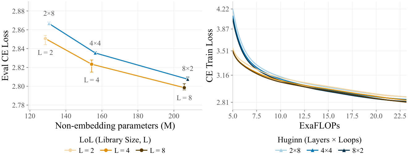
All of these are reported, from the paper:
- Against looped models (Figure 5): at each matched size, LoL's evaluation loss is a little below Huginn's, by about 0.01-0.02 nats. LoL's seed-to-seed spread is wider, which the authors attribute to different paths being explored under different router initialisations.
- Against MoE (Figure 6): at a 3:2 sparsity ratio (MoE with three experts per layer and two active; LoL with 24 experts over 16 depths), the MoE ends slightly lower, 2.75 against 2.8. To match compute, the LoL model's own prelude and coda are MoE layers too (paper, Section 4.3).
- At 1B on math (Figure 4, Table 1): LoL with against a dense model and a sliding-window dense model at matched FLOPs, about 90 ExaFLOPs.
| Model | ARC-E | ARC-C | HellaSwag | PIQA | GSM8K |
|---|---|---|---|---|---|
| Vanilla | 40.8 ± 1.0 | 28.2 ± 1.3 | 31.4 ± 0.5 | 56.6 ± 1.2 | 29.7 ± 1.3 |
| Vanilla (sliding window) | 49.5 ± 1.0 | 28.5 ± 1.3 | 31.3 ± 0.5 | 58.8 ± 1.1 | 27.5 ± 1.2 |
| LoL | 50.3 ± 1.0 | 29.1 ± 1.3 | 31.2 ± 0.5 | 59.7 ± 1.1 | 27.9 ± 1.2 |
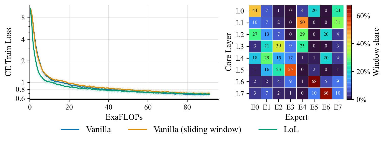
The fair reading is the paper's own: competitive, within about two standard errors, with the full-attention baseline's ARC-Easy score as the outlier. HellaSwag at 31% and ARC-Challenge at 28-29% sit a few points above chance (25%), so at this scale these benchmarks separate the three models very little. Nothing in the paper claims LoL is better per FLOP. It claims parity plus a property dense models lack.
Checking the MoE match from the scripts
The MoE comparison is the one where "matched" carries the most weight, so I recomputed it from shells/lol_vs_moe.sh and the layer definitions (reasoned from the code, not run). Width 1,024; attention is 4.19M parameters per layer; a dense SwiGLU block with hidden width 2,816 is 12.85M.
| MoE baseline | LoL | |
|---|---|---|
| Layout | 24 MoE layers, 3 experts of hidden 1,408, top-2 | 4 + 4 MoE prelude/coda layers (same MoE) + 24 dense blocks, 16 routed depths |
| Stored parameters (non-embedding) | 412.1M | 445.6M |
| Active per token | 308.3M | 308.3M |
| Step cap at batch 26 × 5 × 8 GPUs × 1,024 | 7,269 steps, about 7.7B tokens | 9,393 steps, about 10.0B tokens |
Two observations. The active counts match exactly, because two experts of hidden 1,408 are exactly one dense MLP of 2,816. And at the same 17.3 ExaFLOP budget, LoL's step cap allows about 29% more tokens, because growing makes its early steps cheap. Training stops at the FLOP budget, so the token figures are upper bounds; the paper's own phrase is "approximately 10B tokens for the most efficient model". Read that way, the 0.05-nat gap in the MoE's favour comes with LoL holding 8% more stored parameters and seeing more data. That is not a contradiction of the paper, which claims competitiveness, but it is the honest size of the comparison.
What the paths encode, and forcing them
That property is the paper's real case: the routing path is a discrete, low-dimensional record of what the model did, and you can overwrite it.
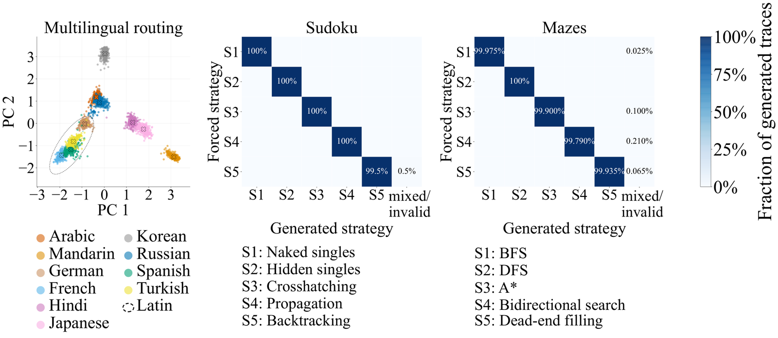
All reported:
- Languages. A model trained on an equal mix of 10 FineWeb-2 languages for 10B tokens. Each window's path, as one-hot experts concatenated over depths and projected with PCA, clusters by language, and the Latin-script languages share paths. Figure 11 shows the clusters forming over training.
- Safety. Trained on FineWeb text labelled safe or unsafe by an existing classifier, with no labels used in training. A ridge probe on a window's router probabilities gets a held-out AUROC of 0.92; on probabilities averaged over a sequence, 0.95. Shuffled labels give chance. These are agreement scores with another classifier's noisy labels, which the appendix states.
- Sudoku and mazes. Five strategies each (naked singles to backtracking; BFS, DFS, A*, bidirectional search, dead-end filling). The strategy token is masked from every part of the network except the router. The authors average router probabilities over validation puzzles to get a "mode path" per strategy, then replace the strategy token with filler and force that path. The forced model produces the requested strategy 99.5-100% of the time on sudoku. On mazes, where all five strategies share one output syntax and differ only in the order cells are visited, it is 99.79-100%.
The maze result is the strongest evidence in the paper. The output vocabulary is identical across strategies, so the path is the only thing selecting the algorithm.
Note the setup, though. The strategy label reaches only the router, so the blocks are trained to depend on routing to know which algorithm to run. The experiment shows a path can carry the strategy. It does not show that the five strategies are built from a shared set of reusable block-primitives, which is what the programming analogy in the thread suggests.
Where the configs and the text disagree
From the shell scripts (shells/*.sh) and configs. All of this is checkable in the repository, and none of it overturns a result, but a reproducer would trip on it.
- Sudoku and maze model size. The paper calls these 360M-parameter models.
shells/sudoku.shandshells/maze.shlaunchn_embd=512,n_head=8, 16 experts, depth 16, with 4 + 4 fixed layers. At width 512 a block is 3.4M parameters, so the 24 stored blocks come to about 82M (reasoned). The run is labelledshape=360mbecause it inherits the 360M shape file and then overrides the width. - Multilingual layout. The paper's 360M setup is 4 prelude layers, 4 coda layers and depth 16.
shells/multilingual.shlaunches 1 prelude layer, 1 coda layer, 33 experts and depth 22. - Input injection. The math, MoE-comparison and backprop-depth runs set
recurrent_input_injection=diagonal: a Parcae-style re-injection of the prelude output at every routed depth, with a learned per-channel decay (DiagonalRecurrentInputInjectioninlol_window.py). The method section does not mention it, though the bibliography cites Parcae. - FiLM. The paper describes per-depth FiLM scale and bias after each norm. In the scripts it is switched on (
depth_expert_film=true) for the Huginn and MoE comparisons only; the default is off. - No weights. The README says to point
CHECKPOINT_*variables at trained checkpoints. None are published, so every number above is reported, not reproduced.
A toy library on CPU
The paper's experiments need 8-GPU nodes. The question I could ask on a 4-core CPU was the one the thread raises: if the task really is "chain primitives in some order", does a learned router discover the primitives and reuse them?
Task. Input: 8 digits mod 10 and a 3-step program. Each step is one of four primitives: inc (add 1 to every digit), rev (reverse), rot (rotate left by one), mul3 (multiply every digit by 3). They do not commute, so order matters. There are 64 programs. I train on 48 and hold out 16, chosen so that every primitive still appears at every step in training. Program tokens are step-specific, so a mean over tokens still says which primitive sits at which step.
Models. Each is a 64-wide, 4-head encoder with 3 block applications:
- dense: 3 distinct blocks in a fixed order;
- looped: 1 block applied 3 times;
- oracle: a library of 4 blocks where step runs block number (primitive at step ), so the routing is handed to it;
- LoL: a library of 4 or 8 blocks with a top-1 router per depth, written to match the released code. That means input , learned softplus noise, a loss-free balancing bias used only for selection, and the update . Tied and untied routers.
- LoL, router-only program: like the paper's sudoku setup. Blocks never see the program tokens; only the router does, through the mean of their embeddings added to its usual input.
Round one (the first version of this article): 3,000 AdamW steps at batch 256, 3 seeds per model, PyTorch 2.14.1 on 2 CPU threads, 2-3 minutes per run. Accuracy is exact match of all 8 output digits on 4,096 fresh examples. Script: one PyTorch file of about 200 lines. The routing is a re-implementation of the code above, not the repo's model, because the repo's model needs FlexAttention and CUDA-scale configs.
What I measured in round one:
- Every model with the program in its input fits the 48 trained programs to 99.4-100%. This task does not reward capacity.
- Held-out programs separate them. Dense: 9.8% (9.2, 10.8, 9.3 over three seeds). Looped: 8.0%. Oracle routing: 44.0% (52.7, 39.2, 40.1). When the right block runs at the right step, the blocks partly become reusable primitives and recombine on unseen programs. (Round two, below, shrinks this gap and finds that reuse is not what drives it.)
- The learned router did not find them. LoL with and a tied router: 4.2% held out (6.8, 4.2, 1.6), below the dense baseline. Untying the router gave 8.3% (3.9, 10.7, 10.4); doubling the library to gave 6.6% (7.4, 12.1, 0.3). None of the nine learned-router runs beat the dense mean by more than a couple of points, and most fell below it.
- The routing tables say why. With they are organised by depth, not by primitive. In tied seed 0, step 2 sends all four primitives to block 2 and step 3 sends all four to block 1. The router found a mostly fixed order with some input-dependent variation, and then the blocks learned to read the program tokens themselves. With the choices vary more with the input, but purity at steps 2 and 3 is 0.34-0.43: the block is not a function of the primitive there either. Forcing the most common block per (step, primitive), the analogue of the paper's mode path, did not rescue held-out programs (0-10.6% across the nine runs).
That matches the paper's own utilisation heatmaps (Figures 4 and 6), where experts "mainly tend to be used in groups of neighboring depths". A router with an option to specialise by depth takes it, because depth is the easiest signal to separate on.
The last pair of runs copies the paper's sudoku setup: the program reaches only the router, so the blocks can only learn which primitive to apply through the path they are on.
- That helps, unevenly. Held-out accuracy rises to 14.8% with a tied router (0.4, 28.8, 15.1) and 16.5% untied (18.7, 1.8, 29.0). Training accuracy also drops: one tied seed reaches only 67.6% on the trained programs.
- The path carries the program, but not as one block per primitive. Purity stays at 0.45-0.72. The router spreads the program across combinations of blocks, a distributed code that works for most trained programs and transfers to some new ones.
So the toy reproduces the paper's direction: hide the task from everything but the router and the path has to carry it. It also shows how far a learned path stays from the clean one: 15-16% against 44.0%, with a seed-to-seed spread of about 28 points.
Round two: the toy again, and two ablations
Round one ended on a reasoned guess about why the router fails, and on a single training setup. For this update I went back to test both. Everything in this section is measured.
First, the rerun did not reproduce round one's gap
The round-one script was not kept. I rewrote it from the description above: same task, same 48/16 split, same widths, the same 3-step encoder and the same routing rule, now with the optimiser written down (AdamW at , 100 warmup steps then cosine decay, weight decay 0.01, gradient clipping at 1.0). Each run uses one CPU thread with two runs side by side, PyTorch 2.14.1, about 4-5 minutes for a top-1 model and about 14 minutes for one that runs every block at every depth. Before adding anything I reran the three models the conclusion rests on, then varied the learning rate and the weight decay.
Held-out accuracy, mean over seeds (trained programs: 99.9-100% for every model in every row):
| Setting | Dense, fixed order | Routing given, by primitive | Learned router (as in the code) |
|---|---|---|---|
| Round one (script lost) | 9.8% | 44.0% | 4.2% |
| Round two, lr 3e-3, wd 0.01, 5 seeds | 25.5% (13.9-33.8) | 38.4% (29.8-49.0) | 12.3% (2.9-20.7) |
| Round two, lr 1e-3, wd 0.01, 3 seeds | 12.8% | 19.4% | 9.0% |
| Round two, lr 3e-3, wd 0.1, 3 seeds | 23.8% | 40.5% | not run |
The ordering held in every row: routing given by primitive beats the dense model, and the dense model beats a learned router. The size of the gap did not hold. Round one put the given routing 34 points above dense; round two puts it 7-17 points above. The dense baseline in particular moves with the optimiser, from 9.8% to 25.5% between two scripts that differ only in details I did not record the first time. So the round-one sentence "the blocks partly become reusable primitives" overstated the effect. The direction is reproducible; the 44-against-10 contrast is not.
Experiment 1: which kind of path transfers
The paper's thread frames the idea as chaining a few primitives in different orders. The toy can take that apart, because I can hand the model any routing I like and see which kinds help on unseen programs. Five schemes, all with routing given and nothing learned about the order:
- No routing: the dense model, three distinct blocks in a fixed order.
- Shared, by primitive: four blocks; every step runs the block numbered by its primitive. This is the round-one oracle.
- One block per (step, primitive): twelve blocks;
incat step 1 andincat step 2 are different blocks, so no block is ever reused across depth. - Shared, relabelled per step: the same four blocks, but steps 2 and 3 use a different primitive-to-block map from step 1. Each block still has a consistent job at each step; it just has a different job at different steps.
- Shared, by program id: four blocks, and each of the 64 programs gets a fixed random path that has nothing to do with its primitives. The held-out programs get paths too, so the router's choice is still a deterministic function of the input.
What I measured (held-out, lr 3e-3, wd 0.01):
- By program id: 0.0% in all three seeds, while fitting 99.7-100% of the trained programs. A path that names the program rather than describing it is a lookup table, and a lookup table has no entry for a new program. Readable, steerable paths are not enough; the path has to be built from the task's parts.
- Relabelled per step: 15.2% (6.2, 18.1, 21.3), below the dense model. Same blocks, same parameter count as the shared oracle at 38.4%. Making a block mean
incat one depth androtat the next costs more than half of the benefit. - One block per (step, primitive): 60.0% (40.4, 76.4, 63.3, 64.0, 55.8), the best of anything I ran. It has three times the parameters (603k against 203k), but capacity is not what the task rewards: every model here fits the trained programs, and the dense model has the fewest blocks of all.
The third result is the one that matters for LoL's framing. In this toy, what transfers to new programs is a path that follows the program's structure. Reusing one block across depths is not where the benefit comes from; it is a constraint that costs accuracy, because the shared inc block has to work on hidden states from three different depths. A library smaller than its depth buys parameter efficiency, which is the looped end of the paper's dial. It does not, on this evidence, buy composition.
Experiment 2: is it the router's gradient?
Round one's explanation was that the router only learns through , the weight of the block it already picked, so it never hears that a different block would have helped. The code reading above adds a second suspect: the balancing bias is shared across depths, so a router that gives each depth its own block is perfectly balanced. Both can be tested. Five ways to train the same tied router, three seeds each (five for the first):
- As in the code: top-1, update scaled by , learned noise, one balancing bias for all depths.
- + sequence balance loss: adds DeepSeek-V3's per-sequence balance term at 0.01, the coefficient the Huginn-comparison runs use.
- Balance per depth: one balancing bias per depth instead of one for the core, so every depth has to use every block.
- Soft mixture in training: every block runs at every depth and the update is , so the router gets a gradient for every block, picked or not. Top-1 at test.
- Gumbel-softmax, annealed: every block runs, weighted by a Gumbel-softmax whose temperature falls from 1 to 0.1 over training, so training ends close to a hard choice. Top-1 at test.
To read the routing, I use two numbers per run, averaged over the three steps. Separation is how well the chosen block identifies the primitive: the share of examples whose block's most common primitive is their own. It is 0.25 when blocks ignore the primitive and 1.0 for the oracle. Depth concentration is how much each block is owned by one depth: the share of each block's use that falls at its busiest step. It is 1/3 when blocks are spread evenly over the three steps and 1.0 when every block belongs to one step.
What I measured:
| Router training | Held-out, top-1 | Separation | Depth concentration |
|---|---|---|---|
| As in the code (5 seeds) | 12.3% | 0.46 | 0.59 |
| + sequence balance loss | 12.4% | 0.46 | 0.41 |
| Balance per depth | 11.2% | 0.46 | 0.35 |
| Soft mixture in training | 0.2% (15.1% if kept soft at test) | 0.47 | 0.54 |
| Gumbel-softmax, annealed | 1.3% (17.5% if kept soft at test) | 0.36 | 0.67 |
- Balancing per depth did what it was meant to and did not help. Depth concentration fell from 0.59 to 0.35, almost the uniform 1/3: blocks were no longer reserved for one step. Separation stayed at 0.46. The router stopped organising by depth and did not start organising by primitive. Held-out went from 12.3% to 11.2%.
- The sequence balance loss had the same effect, more weakly: concentration 0.41, separation 0.46, held-out 12.4%.
- Giving the router a gradient for every block did not find the primitives either. The soft mixture fits the trained programs with its mixture intact (100% in all three seeds), but its top-1 version gets 4.0-9.4% of the trained programs right: the mixture is a different model from its argmax. Kept as a mixture, it scores 15.1% held-out (18.3, 16.4, 10.6), below the dense model at 25.5%, with separation 0.47. The annealed Gumbel run does the same thing more sharply: kept at its final temperature it scores 17.5% held-out (12.3, 17.9, 22.4), and its routing is the most depth-bound of all (concentration 0.67, separation 0.36). In its seed 0, step 1 sends every primitive to block 2 and block 2 is never used again. Its top-1 version fits between 0.7% and 88.9% of the trained programs depending on the seed.
So neither suspect explains the failure on its own. Separation sat between 0.34 and 0.51 in every run of every scheme, against 1.0 for the routing that transfers. Reasoned, not measured: every one of these models fits the 48 trained programs, so the training loss cannot tell a compositional routing apart from any other routing that fits. Only the held-out programs can, and the router never sees them. A learned router finds a routing that works on what it was trained on. Nothing in a top-1 gate, soft or hard, balanced globally or per depth, prefers the one that factorises the task. The paper's sudoku and maze runs get structure into the path by a different route: the strategy label is visible to the router and to nothing else, which forces the path to carry it. Round one's router-only runs (14.8-16.5%) were the toy's version of that, and they were the only learned-router configurations whose mean beat the dense baseline in round one.
What it costs
- Local attention in the core. Windows of 128 tokens with a stride of 64, inside a 1,024-token context. Whatever crosses a long distance has to cross in the prelude or the coda.
- Batching. Different windows run different blocks at the same depth, so a batch becomes a grouped dispatch, like MoE. The code has a
grouped_window_dispatchpath for this and compiles it withtorch.compile. - No cached decoding in the release. The
inferencepath re-runs the prelude and core over the full sequence, and nothing inmodel/keeps a KV cache (grep forkv_cache,past_key,use_cachefinds none). A decode-time implementation would need a cache per (depth, window, chosen block). Because a window's route depends only on earlier windows, it is fixed once the window begins, which makes such a cache possible. - Seed variance. Reported: wider loss spread across seeds than Huginn, because different seeds explore different paths.
What I could not check
- Nothing the paper trained. No checkpoints are published, and every 360M and 1B run is an 8-GPU job. Every loss, benchmark, AUROC and confusion-matrix number above is reported, not reproduced.
- The released code itself. I read it and quoted it, but I did not execute it: it needs FlexAttention,
torch.compileand CUDA-sized configs, and this sandbox does not run cloned third-party training code. The toy re-implements the routing rule from the code, not the code. - Windows and stride. The toy has one window per sequence, so it says nothing about strided window attention, the local-attention cost or the first-window rule. Those claims rest on the paper and on the formula.
- Growing, truncated backprop, FiLM and input injection. The toy uses none of them. Any of the four could change how a router learns, and the paper's main runs use some of them (see the config list above).
- Scale. The toy has three steps, four primitives and 200k parameters. A router that fails to find primitives at this scale could find them at another, with more data, more depth or a different task. My result is that it did not here, under several training schemes, not that it cannot.
- Seed variance. At three to five seeds per setting, the held-out numbers swing by 20 points or more within one model. The orderings I state held in every seed-averaged comparison I ran; individual gaps of a few points are inside that noise.
Where this sits
The paper's related work places it between two lines (reported, from its Section 2):
- Parameter sharing across depth. Universal and looped transformers reuse one block or a small stack; MoEUT makes the looped block itself a mixture of experts. On this site, Huginn and Ouro, SMELT (does looping pay for its FLOPs?), LOOM (looping more than twice without router collapse) and virtual logic depth (looping buys reasoning, not knowledge) cover that side.
- Routing over depth. Mixture-of-Depths lets tokens skip a layer; Mixture-of-Recursions picks how many times a token loops; UniPool shares one MoE expert pool across layers; Mixture of layers with hybrid attention routes through small transformer layers instead of MLPs. The paper calls Gong et al.'s Mixture-of-Modules (EMNLP 2024) the closest: it also assembles a forward pass from shared modules, but adds reuse to a pretrained model, uses top-k with k above one, and averages the selected attention weights to avoid the query-key mismatch that LoL avoids with windows.
LoL's distinct choices are the combination: whole blocks rather than MLPs, one global library for every depth, top-1 per window, and window boundaries that shift with depth. The looped transformer and mixture of experts pages describe the two ends of its dial, and ALoDLM is the adaptive-depth cousin: it varies how many loops a token gets, not which layer runs.
What the paper shows, as reported: a model with input-dependent layer order trains stably at 360M and 1B, matches looped, dense and MoE baselines closely, and exposes a path you can probe and overwrite. The maze result is the evidence that a path can select an algorithm.
What it does not show, and what my toy suggests is hard: that the blocks become reusable primitives which recombine for unseen tasks. In the toy, a routing handed to the model that follows the program's primitives beats a dense model on unseen programs in every setting I tried (by 7-17 points in round two), and a routing that names the program instead of describing it transfers nothing. A learned router, trained five different ways, never got its blocks to line up with the primitives (separation 0.34-0.51, against 1.0) and never beat the dense model on average. The best routing I found reused no block across depth at all, which says the benefit comes from structure in the path, not from reuse.