CRAM: a 1985 Hopfield-Tank energy that trains in 42 ms, and what its 1,000× actually measures
mdjsonmcp2026-11-16 · 28 min · reasoning · looped-transformers · small-models · benchmarks · neurosymbolic
A 2:38 narrated explainer, drawn in code. Every number and picture in it is this article's own; the sources are below.
› transcript
What if AI inference could become a thousand times faster, using physics from the nineteen eighties? That's the post. Here's the paper. Hi, I'm Merrow! CRAM takes an energy from nineteen eighty-five, learns its costs from solved puzzles, and reasons by rolling downhill. Clamp the clues of a Sudoku. Fill every other cell at random. Now walk downhill on an energy. When any chain's energy falls below a threshold fitted from the training solutions, the search stops. Here is the energy, hand-set. Every pair of cells in the same row, column or box that holds the same digit costs one unit. Move one cell at a time to its cheapest digit, and the board parks in a valley with clashes left. No single change helps. So shake it. Pick a clashing cell, redraw its digit with a little temperature. Sometimes the energy goes up. Then it finds the floor. A valid board has energy zero, so the search knows when it is done. Training learns the costs. Pull down the energy of each solved board. Push up the boards one cell away. No search is unrolled, so nothing is backpropagated through time. Same energy, different objectives. Pseudolikelihood reaches ninety-nine percent in forty-eight milliseconds. Backprop through one step takes four point four seconds. Full backprop through time never gets there. The learned weights are the rules. Positive costs on exactly the eight hundred and ten pairs of cells that share a row, column or box. My own laptop fit found the same. These are training times, on one H two hundred. Sudoku trains about a hundred thousand times faster than the quickest baseline. Maze, fifty-five thousand. The thousand comes from one row: N-Queens, against HRM. And CRAM is timed warm. Charge it the start-up the baselines pay, and that row lands right around a thousand. The post promised faster inference. The paper measures training time, and inference in counted operations, not seconds. No special hardware anywhere. Then the authors set the weights by hand. One number solves every Sudoku in the test set. Three solve every maze. A perfect score on these benchmarks shows a few pairwise rules, nothing more. The speed is real, and the benchmarks are too easy. CRAM proves both at once. An old energy, learned in milliseconds, and a warning about Sudoku. Thanks for watching! Every source is in the full article. I'm Merrow. Bye!
Why read this
Hightop 30%The 1,000× traced to one N-Queens row, the learned Sudoku costs read from the checkpoint, and the recipe rebuilt on a laptop CPU in 0.55 s.
- Checked against the source
- Runs on a consumer GPU
- A lasting reference
LLM architectureApache-2.0Research paper
How this was scored
- Is it new?
- 2 of 3: A real new idea, method or capability
- Can I trust it?
- 3 of 3: Reproduces the headline result, or shows from primary files it is wrong
- Can I run it?
- 2 of 3: Open code or weights with real limits
- Will I understand it?
- 2 of 3: Mechanism from first principles with figures
- Can I act on it?
- 2 of 3: A concrete recipe, numbers or comparison
- Will it last?
- 2 of 3: A reference for a year or more
- Does it affect many?
- 1 of 3: A specialist community
- Only here?
- 2 of 3: A teardown or measurement few others did
Score 72 of 100, ranked 109 of 748 rated articles. Each question is answered 0–3 by hand, and a 3 is rare. How articles are scored
On 15 November a post on X asked: "What if AI inference could become 1,000× faster using physics from the 1980s?" It introduced CRAM, "an energy-based model inspired by Hopfield networks", and listed what it called reported results: 1,000× faster training, 280× lower compute, nearly 100% Sudoku accuracy from 30 training puzzles, no backpropagation through time. Five hundred people liked it.
The paper is Classical Energies Learn to Reason 1,000× Faster than Looped Models by Benjamin Hoover, Hugh Blayney and James Whittington of Prefrontal in London, with a company post and code. It is a better piece of work than the post makes it sound, and a narrower one. The post's opening line contradicts its own bullet list. The 1,000× is training wall-clock. The inference number is 282× fewer counted FLOPs, not seconds. Nothing runs on analog, optical or thermodynamic hardware; every number comes from one NVIDIA H200 running PyTorch and Triton. And the "physics from the 1980s" is not a metaphor for some new device. It is a specific energy function that John Hopfield and David Tank wrote down in 1985, with its weights learned instead of set by hand.
Compact Reasoning Associative Memory: Classical Energies Learn to Reason 1,000× Faster than Looped Models
- license
- Apache-2.0
- branch
- main
- forks
- 6
- open issues
- 8
- source
- 1.6 MB
- commit date
- 2026-11-13
GitHub REST API, 2026-11-16 — branch, commit, commitDate, createdAt, description, forks, languages, license, openIssues, pushedAt, stars
I read the paper, the post and the repository, read the trained Sudoku weights straight out of the checkpoint files, recomputed every speedup from the authors' own run records, and wrote a small NumPy version of the recipe to run on my laptop. The rest of this piece is what that turned up.
Which 1980s physics
Four pieces, all from the 1980s, and CRAM uses all of them.
The energy. In 1982 Hopfield showed that a network of binary neurons with symmetric weights has a scalar energy that never goes up as neurons update (Hopfield 1982). It is an Ising spin glass with learnable couplings. Stored patterns sit at the bottoms of valleys, and a corrupted pattern rolls down into the nearest one. That is associative memory, and it is where the name comes from: Compact Reasoning Associative Memory.
Optimisation as an energy. In 1985 Hopfield and Tank turned the trick around (Hopfield and Tank 1985). Instead of storing memories in the weights, they designed weights so that the low-energy states of the network are the good answers to an optimisation problem: a tour of cities, later a filled-in Sudoku (Hopfield 2008). Constraint violations cost energy; a valid answer costs none.
The probabilities. The same year, Ackley, Hinton and Sejnowski read the energy as a Boltzmann distribution, , and showed how to learn the weights from data: lower the energy of what you see, raise the energy of what the model would otherwise produce.
The sampler. And in 1984 Geman and Geman gave the move that samples from such a distribution one variable at a time, Gibbs sampling, with a temperature that can be lowered as the search goes on.
CRAM writes the Hopfield-Tank energy in the form Peterson and Söderberg gave it in 1989 for neurons with states instead of two. A puzzle has cells, each with possible values (81 cells and 9 digits for Sudoku). The state is a belief array , one softmax distribution over values per cell, and the energy is
is a table of costs, one entry for every pair of values that cells and could take together. is a cost per value at cell . When every cell commits to one value the entropy term is zero, and the energy is just the sum of the pair costs of the chosen values plus their input costs. Sudoku in this language: a cost of one whenever two cells in the same row, column or box hold the same digit, zero for everything else. A valid board has energy zero, and nothing can go lower.
The learned part is the tables. For Sudoku the model is given no rows, columns or boxes; every one of the 3,240 cell pairs gets its own free table, 263,169 parameters in all with the input costs, all starting at zero. Whatever structure ends up in them comes from solved puzzles.
Reasoning is rolling downhill, with some shaking
Given a puzzle, CRAM clamps the clue cells and minimises the energy over the rest. The paper derives the continuous version first. Each free cell has a logit vector with , and the logits follow the negative gradient of the energy:
With that is one layer of a recurrent network applied over and over: the same shape as a looped model, except that each pass is a descent step on a known function. Appendix E proves the energy cannot increase in continuous time. That gives the stability looped models bolt on with fixed-point losses, and a natural stopping signal they bolt on with halting heads.
That update is not what produces the paper's tables, though. Deterministic descent stops at the first valley it reaches, and Sudoku-Extreme has plenty of valleys with two or three conflicts left in them. What actually runs is a focused Gibbs search over committed digits (App. C.3.1):
- Start four independent chains from uniformly random digits in the free cells.
- Each move, pick a random free cell whose local energy is high (any free cell if none is), and redraw its digit from .
- Lower the temperature geometrically from to over 524,288 moves, then restart the schedule. is the mean positive learned cost, so the temperature is in units of "one conflict".
- Stop the moment any chain's energy is at or below a threshold fitted from the training solutions: the highest energy any training solution had, plus .
A move touches one cell, so the kernel keeps every cell's field (the cost of each digit given its neighbours) in memory and updates only the cells coupled to the one that moved. On the GPU each chain is one warp. Step 3 is simulated annealing in all but name.
The threshold matters more than it looks. Because a valid board's energy is known in advance, the search knows when it is done, and on 412,786 test puzzles it never once stopped on a wrong board (Table 4). It does fail: 51 of 1,238,358 searches across three seeds ran out of budget, which is where the 99.996% comes from. The five baselines with a halting rule (HRM, TRM, EqR, TRMP, EBR) each stop on a wrong answer on between 0.05% and 3.54% of the puzzles it stops on.
The widget below runs that search in your browser on a real Sudoku-Extreme puzzle, with the hand-set energy (cost one per clashing pair) in place of the learned one. Set the temperature to zero and watch plain descent park the board in a valley with a few red cells left. Give it a little temperature and it climbs out.
In my own runs of that loop (outside the browser, at a fixed temperature of 0.35 conflicts with focusing on), the easiest Sudoku-Extreme puzzle I tried took between 13,723 and 21,046 moves across three random starts, and puzzles rated 4 and up often needed more than 300,000. Those numbers are for one chain with no annealing schedule; they are there to show the scale of the search, and they say nothing about the GPU kernel's speed.
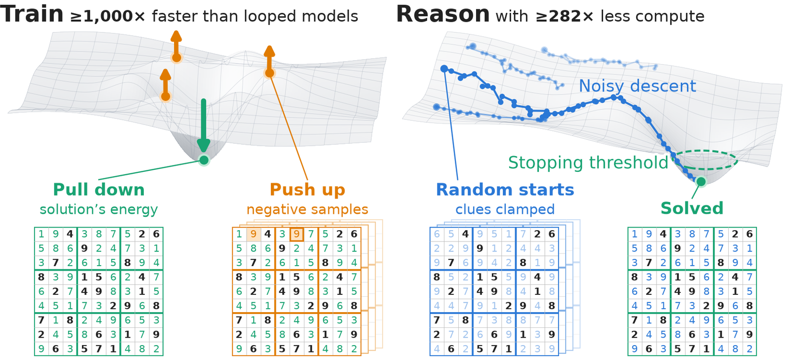
Training without unrolling anything
A looped model like HRM or TRM learns by running its loop, comparing the final answer with the label, and backpropagating through the steps (truncated BPTT). Training cost grows with the number of steps it differentiates through, and the gradients through a long loop are unstable.
An explicit energy offers a way around that. The maximum-likelihood gradient of a Boltzmann distribution has two terms:
Lower the energy of real solutions; raise the energy of what the model currently likes. Neither term differentiates through a search. The second term needs samples from the model, which is expensive, so CRAM uses Besag's 1975 pseudolikelihood instead: for each free cell of a training solution, compare the solution with the eight boards that differ from it in that one cell only.
Every energy term not involving cell cancels inside the sum, so this is a plain softmax cross-entropy per cell, with logits that are minus the local costs of each digit given the true neighbours. No inference, no sampling, no loop. One update is one batched einsum over the training boards. The Sudoku fit is 32 full-batch updates of SGD with momentum and a cosine learning rate, an L1 soft-threshold after each step to zero out costs the data does not support, and a fresh random relabelling of the digits on every update as augmentation. That is the whole training run, and it takes 42 ms on an H200.
The paper isolates how much of the speed comes from the objective. Figure 4 and Table 7 train the same energy twelve different ways. To reach 99% on 512 development puzzles, pseudolikelihood takes 48 ms, minimum probability flow 0.21 s, one-step BPTT 4.4 s and contrastive divergence 33 s. Full BPTT through ten relaxation steps never gets there: after 3,840,000 updates, about five hours, it solves 48.8% of the test puzzles.
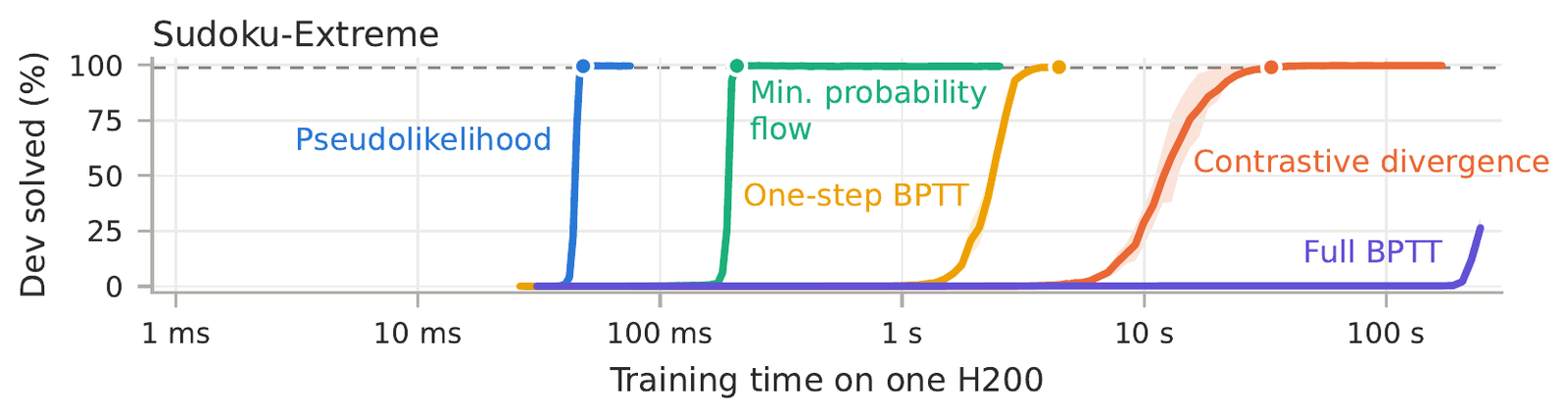
So on the same 263,169-parameter energy the objective alone is worth about 90× (4.4 s against 48 ms). The rest of the gap to the looped models is size: those models have millions of weights and train for hours, and CRAM has a few thousand nonzero costs and trains for 32 steps.
The weights are the rules
Because every cost has a meaning (how much do cells and dislike holding digits and together?), you can read the trained model. The paper says that in every run CRAM put positive equal-digit costs on exactly the 810 pairs of cells that share a row, column or box, and left everything else zero.
I checked that against the three released Sudoku checkpoints. The files are PyTorch zips; I read the raw float32 storages without unpickling anything, indexed the 3,240 pairs in upper-triangle order as the code does, and compared each with the Sudoku peer graph. (81 cells times 20 peers, halved, is 810.)
| seed 0 | seed 1 | seed 2 | |
|---|---|---|---|
| nonzero parameters | 7,716 | 7,750 | 7,761 |
| peer pairs with positive cost on all 9 equal digits | 810 of 810 | 810 of 810 | 810 of 810 |
| range of those costs | 0.493 to 1.317 | 0.482 to 1.324 | 0.491 to 1.315 |
| nonzero costs between different digits | 0 | 1 | 0 |
| small negative equal-digit costs on non-peer pairs | 426 | 458 | 471 |
| largest of those, in magnitude | 0.098 | 0.084 | 0.084 |
The headline holds exactly: every positive cost is a real Sudoku constraint, and every real constraint got a positive cost, in all three seeds. "All other costs zero" is loose. Each seed keeps a few hundred tiny negative costs between cells that do not interact, all on equal digits, the largest about a fifth of the smallest real constraint. They are already inside the paper's 7.7K parameter count, and they do not stop the search; they are what an L1 penalty leaves behind after 32 steps.
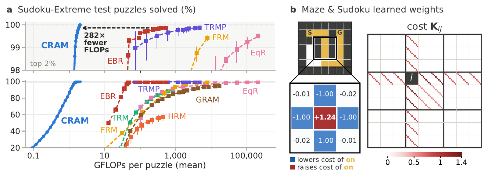
The maze model is smaller still. Maze-Unique gets one cost table per neighbour offset in a window, shared across all 900 cells: 18 numbers. The learned kernel makes an open cell with only one open neighbour cheaper to switch off, and the search starts with every open cell on. Each move turns off one dead end. That is dead-end filling, a textbook algorithm that solves any maze with a unique path, recovered from 1,000 solved examples. It also explains a detail in Appendix C.4: an exact solver fails on this energy, because the empty board has lower energy than the solution, and only the descent from "everything on" lands on the path.
The same recipe on a laptop
The training step is simple enough to write from scratch, so before running the authors' code I wrote my own. cram_toy.py is about 200 lines of NumPy: the pairwise energy, pseudolikelihood with digit relabelling, SGD with momentum 0.5 and a cosine schedule from a learning rate of 540, an L1 soft-threshold of , and a pure-Python focused Gibbs search with the paper's temperatures and threshold rule. The data is 1,000 solved boards from the head of the Sudoku-Extreme train.csv and 40 test puzzles sampled from the head of test.csv, both fetched by HTTP range request. The heart of the fit:
# cram_toy.py: one pseudolikelihood update over every training board
Y = np.eye(D, dtype=np.float32)[y]                         # (boards, 81, 9) one-hot, digits relabelled
G = np.einsum('ijac,bjc->bia', S, Y, optimize=True) + B    # local cost of each digit at each cell
z = -G; z -= z.max(-1, keepdims=True)
q = np.exp(z); q /= q.sum(-1, keepdims=True)               # p(cell i = a | all other cells true)
g = (q - Y) * fr[..., None] / nfree                        # cross-entropy gradient, free cells only
dS = -np.einsum('bia,bjc->ijac', g, Y, optimize=True)
On my M1 Max the fit took 0.55 s, NumPy with its default BLAS threads. It ended with 7,769 nonzero parameters, positive equal-digit costs on exactly the 810 peer pairs and nowhere else, costs between 0.488 and 1.342, one stray off-diagonal entry and 478 small leftovers on non-peer pairs. That is the same model the checkpoints contain, to within the scatter between their seeds, learned by code that shares nothing with theirs except the recipe in Table 5.
The search is where Python hurts. With four chains run one after another and a budget of 2,000,000 moves per puzzle, the focused Gibbs search solved 37 of 40 Sudoku-Extreme puzzles and stopped on a wrong board zero times; the median solved puzzle took 281,476 moves, and the 40 puzzles took 259 s. With the temperature set to zero, plain descent from the same starts solved none of the 40: every chain parked in a valley with conflicts left. I would not read much into the 37: the paper's budget is FLOPs per puzzle, far more moves than my Python loop can afford, and three misses in 40 is what a short budget looks like. The fit and the learned structure are the parts I reproduced.
The authors' code on an RTX 3090
I also had the repository at commit 62bbe83 run on a consumer card, an RTX 3090 in a box I use for this kind of check. Three things came out of it.
The Sudoku fit reproduces. sudoku.py diag fits the paper's three training splits and three no-relabelling variants; its own timer puts each fit loop at about 0.04 to 0.05 s on the 3090 (0.046 s for split 2), roughly the H200's 42 ms. The whole command, Python start-up and imports included, took 4.74 s of wall clock. The weights it wrote for split 2 have the same statistics as the released seed-2 checkpoint I read by hand: 7,290 positive peer costs from 0.4909 to 1.3146 and 471 small negative non-peer costs. The variant without digit relabelling is a useful contrast: it also puts positive costs on all 810 peer pairs, but keeps hundreds of spurious off-diagonal and input costs, and the repository's diagnostic flags hundreds of thousands of single-cell changes it scores wrongly. The augmentation does real work.
The Maze-Unique fit, 20 updates, timed its loop at 0.41 s; the command took 6.52 s of wall clock. That is slower than the H200's 0.13 s, and well inside "under a second".
Then I scored the paper's seed-0 Sudoku checkpoint on the 10,000 development puzzles with checkpoints/evaluate.py. It solved all 10,000 with no wrong stops and no exhausted budgets, which matches the recorded run. The repository's own check still reported a mismatch: the mean count was FLOPs per puzzle against a recorded , about 6% more. The script says a dev run "must reproduce in every field", so the search is not bit-exact across GPUs; the outcome is, and 6% does not move the 282×. The whole batch took about 226 s on the 3090, about 23 ms per puzzle averaged, though the last minutes are a long tail with one or two hard puzzles running alone. That is the only wall-clock inference number I have, and it has nothing to compare against.
Where "at least 1,000×" comes from
Table 2 reports CRAM's fit time against seven looped baselines (HRM, TRM, GRAM, EqR, FRM, TRMP, EBR), and Table 3 against four of them, retrained by the authors with their own code on one H200. The rounded table cells are dramatic: 0.04 s for Sudoku against 1.2 to 9.0 hours, 0.13 s for Maze against 2.0 to 23.2 hours. The repository has the unrounded records (results/baseline-fit-times.json, results/multi-solution-table.json, and a run record for each CRAM fit), so I recomputed every ratio.
With CRAM timed the paper's way, the smallest ratio on each task is against the fastest baseline to train: about 101,000× on Sudoku (HRM, 4,302 s, against 0.0424 s) and 55,000× on Maze (EBR, 7,255 s, against 0.132 s). Prefrontal's post says "over 50,000x" for those two, which is right. The "at least 1,000×" in the title is set by a different table. On N-Queens 8×8 HRM trained in 59 minutes (3,542.6 s) and CRAM in 2.896 s, which is 1,223×. That one row is the floor of the headline.
Two assumptions sit under it.
Warm against cold. The paper times CRAM warm: the median of seven complete fits that follow a first fit in the same process, so kernel loading and compilation are already paid. Each baseline is one cold fit in a fresh process. Section C.2 says so plainly and gives the reason: CRAM's one-time start-up of 0.2 to 0.9 s is most of a 42 ms fit and a rounding error on a nine-hour one. Fair, but it moves the floor. The run records include cold times: Sudoku's first fit took 0.501 s and Maze's 0.80 s, which still leaves 8,582× and 9,074×. N-Queens is the row that bends. The 2.896 s figure is a re-timed version of the fit that builds the cost matrix with one dense product instead of indexing (App. C.5), and no cold time is recorded for it. The checkpoint folder's own record of the indexing fit, with weights the paper says agree to within , says 5.60 s cold and 4.53 s warm: 632× and 782× against HRM. Add the paper's stated start-up range of 0.2 to 0.9 s to 2.896 s instead and you get 933× to 1,144×. So that row lands at about 1,000×: 1,223× as published, a little either side of 1,000× with start-up added, and 632× to 782× on the released checkpoint's own (slower, indexing) fit, where start-up is not what moves it.
A full schedule against a full schedule. A baseline's fit time is its authors' entire published training schedule, not the time it took to reach some accuracy. HRM trains Sudoku for 40,000 epochs because that is what its released checkpoint used. Nobody measured when HRM first matched CRAM; it never does, at 54.62%. So these are ratios of recipes. That is a reasonable thing to report, and it is a different claim from "the same accuracy, 1,000× sooner".
The ledger below has every row. Switch CRAM to cold to charge it start-up, or to one CPU thread, which the records also include.
The CPU column surprised me. On one thread of a Xeon Platinum 8468 the Sudoku fit took 1.71 s cold and the Maze fit 0.12 s, which for Maze beats the GPU's cold start. Graph coloring is the exception: its cost tables are an affine function of every adjacency token, and on one CPU thread that fit takes about a minute, 41× faster than HRM's GPU run rather than thousands. For the two benchmarks people actually quote, though, CRAM does not need a GPU to train at all.
So the 1,000× is real as a statement about recipes on these benchmarks, with one caveat on one table row. It is not about inference.
The 282× is counted FLOPs
The inference claim is that CRAM matches each looped model's best accuracy on 10,000 Sudoku-Extreme puzzles with at least 282× fewer floating-point operations. The 282× is against EBR, the cheapest baseline at its best: EBR reaches 99.86% at FLOPs per puzzle, CRAM at . Against the others the gap is larger, up to 128,000× against EqR, which runs 128 noisy restarts at depth 64.
How those FLOPs are counted matters.
The convention (App. C.2) counts a multiply-add as 2, every elementwise operation and transcendental as 1, and comparisons, selections, indexing, data movement and random-number generation as 0. That is standard for neural networks, where matmuls dominate. A single-cell Gibbs move is the opposite kind of workload: pick a cell, look up its row, draw a random number, compare against a cumulative sum, scatter updates to twenty neighbours. Much of it is the free part. The repository's results/op-counts.json also records CRAM's count with comparisons: per puzzle instead of , about 1.5× more. That does not dent a ratio of 282, but it shows what kind of count this is.
CRAM's moves run in Triton kernels that the PyTorch FLOP counter cannot see, so its count is a line-by-line hand transcription of the kernel (cram/opcount.py); the baselines were counted automatically at the operator level. The repository makes the transcription checkable, which I appreciate.
And there is no wall-clock inference comparison in the paper at all. The closest thing is in checkpoints/evaluate.py's docstring: scoring all 412,786 test puzzles takes "about 1.5 GPU hours on one H200", and the 10,000 development puzzles "about 5 minutes". That works out to roughly 13 ms and 30 ms per puzzle in a batch. The N-Queens 8×8 checkpoint record has its test search at 12.8 s for 1,240 rows with 20 chains each. Those are small numbers. They are not compared against anything in the paper, so "1,000× faster inference" has no source.
What the energy does buy at inference is adaptive compute. Because the search stops at the threshold, easy puzzles stop early. Binned by the dataset's difficulty rating, CRAM's median compute grows 22× from the easiest bin to the hardest, while FRM spends the same compute on every puzzle and EBR barely varies.
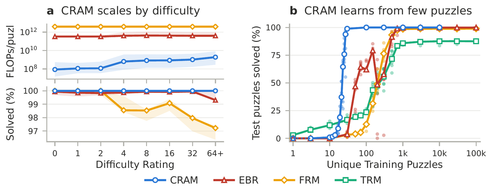
Thirty puzzles, times a hundred
The post's "nearly 100% Sudoku accuracy with just 30 training puzzles" comes from Figure 3b. The paper's words: CRAM "needs an order of magnitude fewer puzzles to reach 98% accuracy than looped models, using only 30 unique puzzles to EBR's 700." Each unique puzzle is augmented with 99 symmetry variants (digit relabelling, transposition, band and stack permutations), so 30 unique puzzles is 3,000 training boards, for every method in that figure. Ninety-eight percent is near enough to "nearly 100%". What stands out is how sharp the curve is: below about 20 puzzles CRAM solves almost nothing, and the paper notes it "converged to many incorrect solutions" there, while TRM does best in the extreme low-data regime and then plateaus.
That sharpness makes sense once you know what is being learned. There are 810 constraints to find, each a statement that two cells never share a digit. Thirty solved boards with relabelling show enough pairs of equal digits in non-peer cells to rule those pairs out, and never show one in a peer pair. A model with the right inductive bias needs very little data to fill in a table of 810 yes-or-no facts.
One weight solves every Sudoku
The result I would put first, and the one the post left out, is in the gray rows of Tables 2 and 3. The authors also set CRAM's weights by hand from each task's rules and ran the same search. For Sudoku that is the identity matrix on the 20 peers of every cell: one unique nonzero value. It solves 100% of the test puzzles, with 19× fewer inference FLOPs than the learned energy. Maze-Unique needs three hand-set values, N-Queens two, graph coloring one, and each solves every test puzzle.
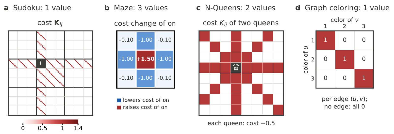
That is a statement about the benchmarks. Sudoku-Extreme, Maze-Unique, N-Queens and these graph-coloring sets are constraint problems whose rules are pairwise between answer cells, so a pairwise energy can represent them exactly. A model that scores 100% on them has shown it can discover a few pairwise rules. The authors say this themselves, more than once: high accuracy here "does not indicate that a model can scale to harder tasks such as ARC-AGI", and the paper ends with a caution against using benchmarks this easy to judge whether looped reasoning scales. I have read several looped-model papers on this site that lead with Sudoku-Extreme, including the Lattice Deduction Transformer, which reported 100% after about 15 minutes on one B200. CRAM reaches 99.996% in 42 ms of training with an 80s energy, and a hand-set version gets there with no training.
The authors do try one step past pairwise. Maze-Hard has loops, so dead-end filling fails, and plain CRAM solves none of its test mazes. Appendix F adds one hidden neuron per open cell whose energy is strictly convex, so it settles to a field that falls off with distance from the goal; the visible pair costs read that field through a small attention. With 29 learned parameters and about half a minute of training, it solves 999 of 1,000 test mazes in each of three runs. That is a nice construction, and the authors are candid that they chose the hidden quantity knowing the task needed distances. Learning what latent to compute, without being told, is the open problem, and nothing here touches it.
Two corrections and a compliment
The core result holds, and I reproduced the part that matters most: a pairwise energy fitted by pseudolikelihood from zero recovers the exact Sudoku constraint graph in about half a second on a laptop, without being told what a row is. The training speed is real and mostly comes from two places the paper is clear about: a model with a few thousand meaningful parameters instead of millions, and an objective that never unrolls the search.
The headline needs two corrections. The 1,000× is training, timed warm, and its floor rests on one N-Queens row that lands at about 1,000× once you vary how it is timed. Sudoku and Maze are comfortably above 8,000× on the GPU, warm or cold, and above 2,500× on one CPU thread. The 282× is FLOPs under a convention that leaves most of a Gibbs move uncounted, with no wall-clock comparison anywhere. And the "1,000× faster inference" in the post is not a claim the paper makes.
I think the paper's real contribution is the benchmark critique, and it is a good one. If one hand-set weight solves every Sudoku-Extreme puzzle, a looped transformer that needs 27 million parameters and an hour of training to reach 55% is telling us about its own inefficiency, not about reasoning. If you build looped or recursive reasoners, read Tables 2 and 3 before you put Sudoku in your abstract. If you were hoping for a new kind of hardware, this is not that; for a real attempt at a chip that samples instead of multiplying, see Extropic's Z1T, and for whether looping helps once you pay for the FLOPs, SMELT and what separates Ouro from Huginn.